Installing JupyterLab Desktop


Figure 1

Apple Silicon Chip


Figure 2

Installation Screen


Figure 3

MacOS Installation Prompt


Figure 4

Installation Screen


Figure 5

JupyterLab download


Figure 6

JupyterLab setup


Figure 7

JupyterLab launch


Figure 8

Bundled Environnment Prompt


Figure 9

JupyterLab Menu Bar


Figure 10

JupyterLab Main Work Area


Figure 11

JupyterLab Left Side Bar


Figure 12

Show File Browser in Menu


Figure 13

JupyterLab Start Session


Figure 14

Launch a New Python3 Notebook


Figure 15

Recent Sessions


Figure 16

Print Working Directory from within Python


Figure 17

Find Settings in JupyterLab


Figure 18

Choose Settings


Figure 19

Default Working Directory Setting


Running and Quitting


Figure 1

Anaconda Navigator landing page


Figure 2

JupyterLab landing page


Figure 3

JupyterLab Menu Bar


Figure 4

JupyterLab Left Side Bar


Figure 5

JupyterLab Main Work Area


Figure 6

Example Jupyter Notebook


Figure 7

Multi-panel JupyterLab


Variables and Assignment


Figure 1

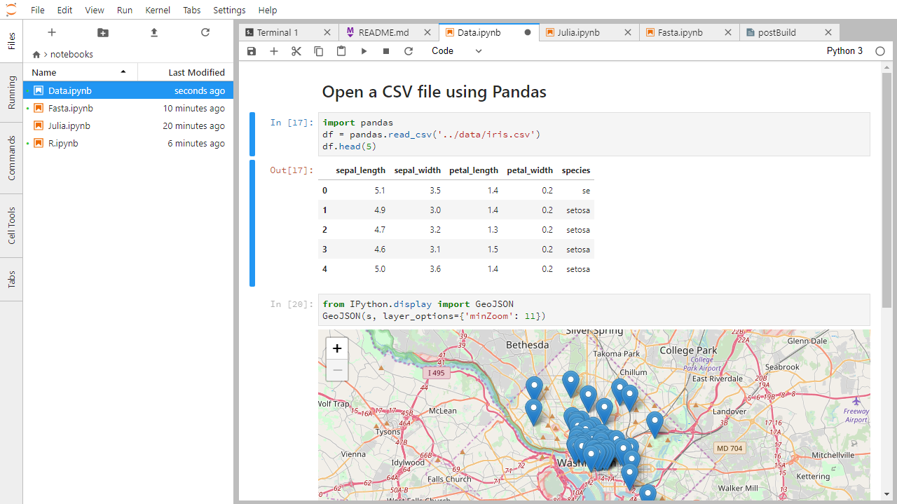
A line of Python code, print(atom_name[0]), demonstrates that using the zero index will output just the initial letter, in this case ‘h’ for helium.
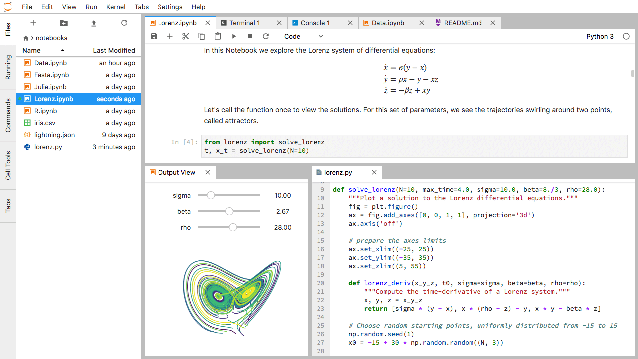
Data Types and Type Conversion


Built-in Functions and Help


Libraries


Reading Tabular Data into DataFrames


Pandas DataFrames


Plotting


Figure 1

A line chart showing time (hr) relative to position (km), using the values provided in the code block above. By default, the plotted line is blue against a white background, and the axes have been scaled automatically to fit the range of the input data.

Figure 2

GDP plot for Australia

Figure 3

GDP plot for Australia and New Zealand

Figure 4

GDP barplot for Australia

Figure 5

GDP formatted plot for Australia

Figure 6

GDP formatted plot for Australia and New Zealand

Figure 7

GDP correlation using plt.scatter

Figure 8

GDP correlation using data.T.plot.scatter

Figure 9

Minima Maxima Solution

Figure 10

Correlations Solution 1

Figure 11

Correlations Solution 2

Figure 12

More Correlations Solution

Lists


For Loops


Conditionals


Looping Over Data Sets


Writing Functions


Variable Scope


Programming Style


Wrap-Up


Feedback