
All in One View
Content from Installing Python and JupyterLab
Last updated on 2026-10-05 | Edit this page
Overview
Questions
- How do I install Python?
- How do I launch JupyterLab?
Objectives
- Download and install Python.
- Install the JupyterLab, Pandas, and Matplotlib packages.
- Organize folders and files on your computer.
- Create a folder to hold the Jupyter notebooks you will create during this workshop series.
Getting Started with Python
In this activity, you will install Python to your personal computer. You only need to install and configure Python once for this workshop, so future lessons will assume that you already have Python installed.
JupyterLab is an application developed by Project Jupyter that enables one to working with Jupyter notebooks, text editors, terminals, and even custom components in a flexible, integrated, and extensible manner.
Installing Python
The easiest way to install Python and JupyterLab will depend on your operating system.
- If you have a Mac laptop, install for MacOS.
- If you have a Windows laptop, install for Windows.
If you encounter an error during the installation process, please flag down an assistant, ask a question over Zoom, or contact your instructor through Canvas if you are working asynchronously.
Installing Python: MacOS
Before installing Python on a Mac, you will need to know the type of processor it has.
Depending on when you bought your laptop, your Mac may have an Apple Silicon chip or an Intel chip. For Python to work correctly, you must install the version that corresponds to your laptop’s chip.
Finding Your Processor Chip Type
- Click on the Apple icon in the top left corner of your screen.
- Select About this Mac.
- Look at the line labeled Chip.
- If your chip name begins with Apple, it is an Apple Silicon processor.
- If your chip name begins with Intel, it is an Intel processor.

Downloading Python
To make installation faster and easier, you will be downloading Python through an environment management tool called Miniconda.
Go to the Anaconda/Miniconda download page.
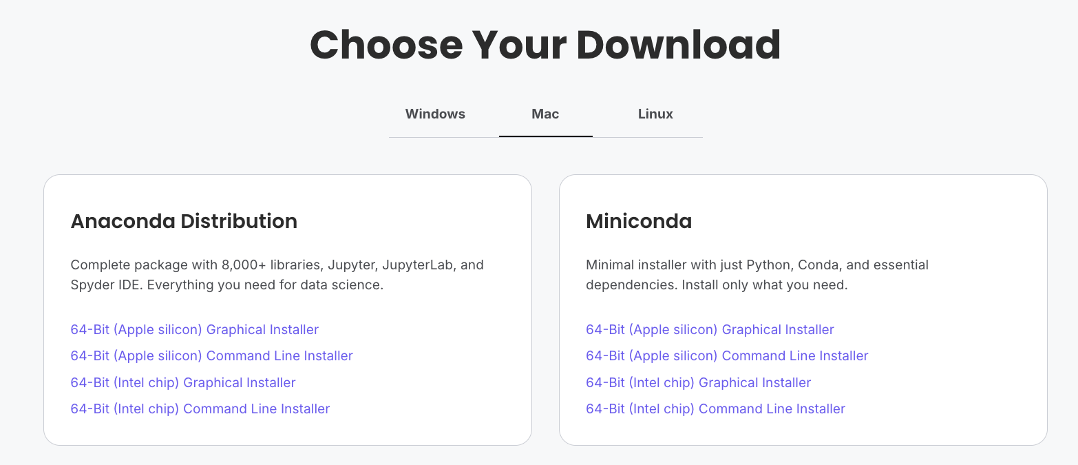
From the Miniconda column, select the Graphical installer download that corresponds to your chip type.
For example, if you have a Mac with an Apple Silicon chip, you should select the 64-Bit (Apple silicon) Graphical Installer.
Double-click to download the file to your computer.
Installing Miniconda
Once the download has completed, double-click the Miniconda .pkg file in your Downloads folder.
A graphical installer will launch.
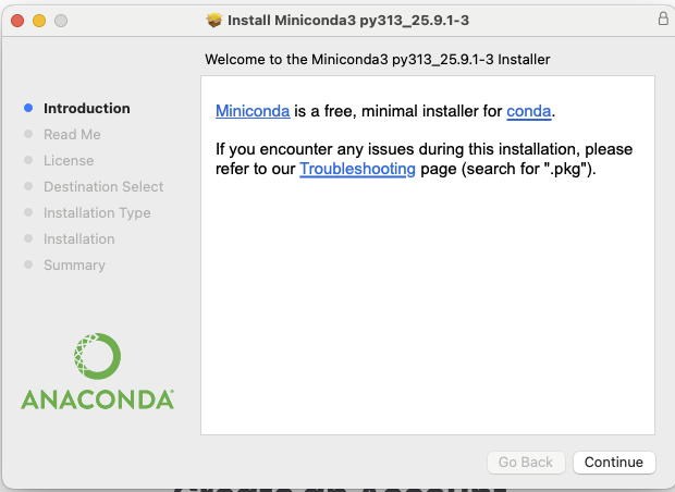
Press Continue to navigate through the installer. Click Agree to the terms of the End User License Agreement.
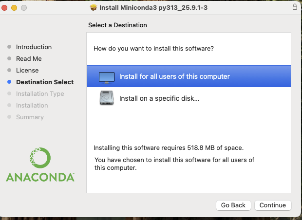
When prompted to select a destination for your Python installation, select “Install for all users of this computer”.
This will install Miniconda (and Python) to your computer. Click Continue.
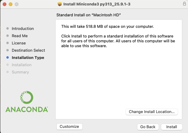
When prompted, click Install.
Wait while Miniconda installs. This should take fewer than 5 minutes.
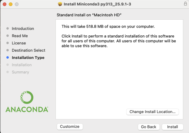
When the installation has finished, close the installer window by clicking Close.
Installing JupyterLab
Look for the magnifying glass icon in the top right corner of your screen. Search for Terminal and click the icon to launch the Terminal application.

The Terminal (or command line) is a special application that allows you to talk to software on your computer through textual commands. Some applications can only be accessed through the command line.
Type the command
conda install jupyterlab pandas matplotlib and press the
Enter key.
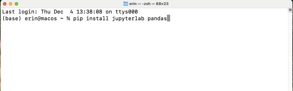
You may be prompted to press the a key twice, followed by the y key. The required software for this workshop will be downloaded from the internet.
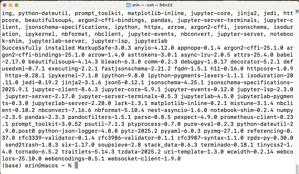
When you see your username followed by a blinking cursor, that means that the terminal is waiting for another command. You are ready to launch JupyterLab.
Launching JupyterLab
Congratulations! You’ve installed JupyterLab. You will not need to perform these installation steps again.
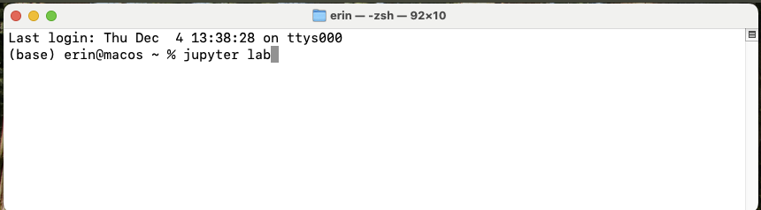
Now, and in the future you can launch Juptyer Lab by doing the following:
- Search for Terminal.
- Open Terminal.
- Type
jupyter labinside the terminal and press the Enter key.
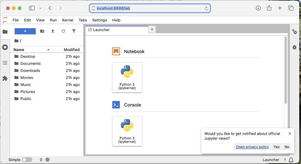
JupyterLab will launch in a new tab in your default web browser.
Installing Python: Windows
Downloading Python for Windows
To make installation faster and easier, you will be downloading Python through an environment management tool called Miniconda.
Go to the Anaconda/Miniconda download page.
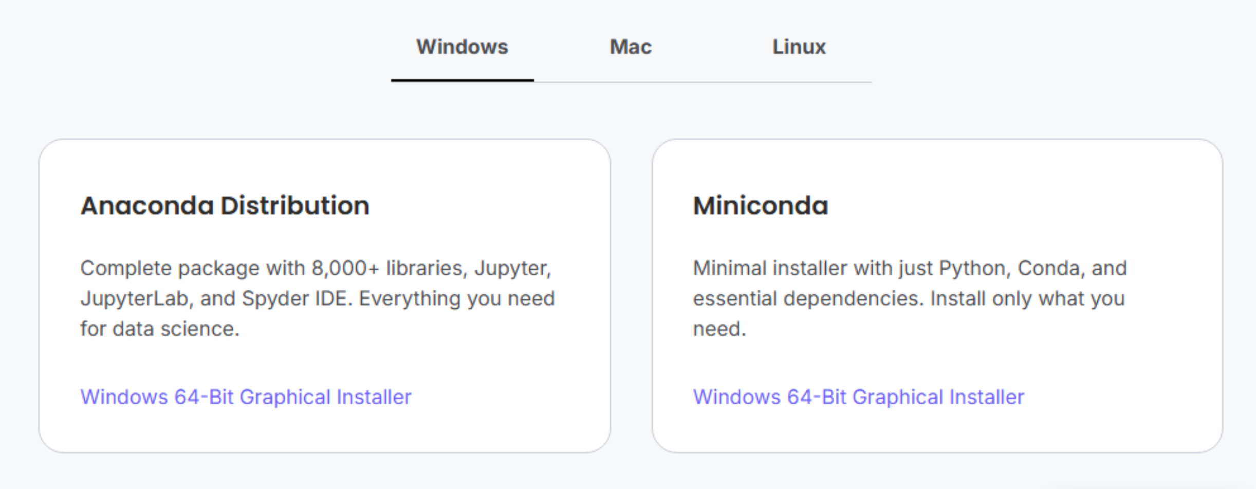
Click the Miniconda link to download the file to your computer.
Installing Miniconda
Locate the downloaded file (likely in your Downloads folder if you did not specify a location) to start the installation process. Double-click it.
You will see an installer like this open.
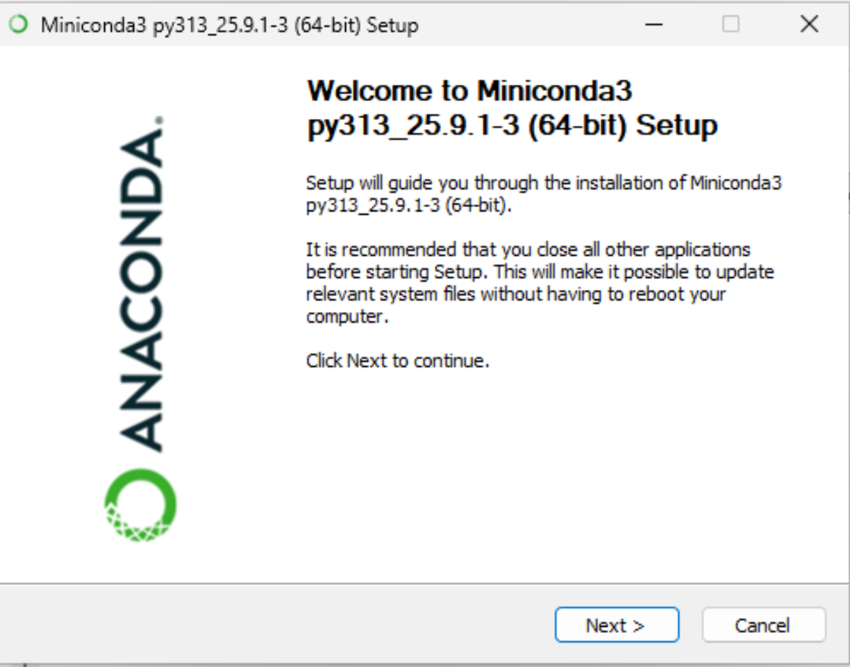
Click Next to proceed to the next screen of the installer.
Read through Miniconda’s End User License Agreement (EULA) and click I Agree to agree to the terms.
You will be prompted to select for which users Miniconda should be installed, either
- Just Me (Recommended)
- All Users
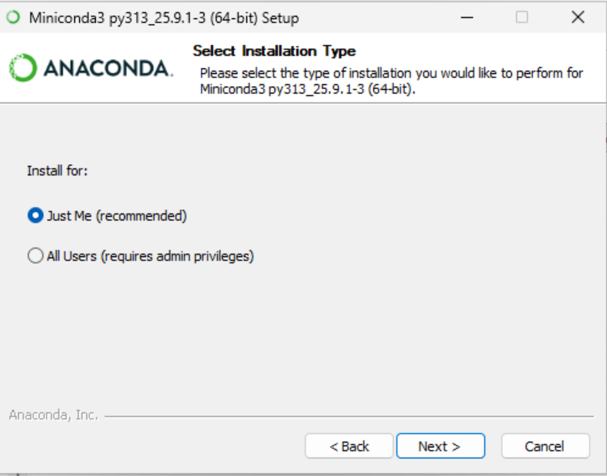
Select Just Me and click Next.
Next, you will be prompted to select where Miniconda should be installed. The default location, in your home directory, is appropriate.
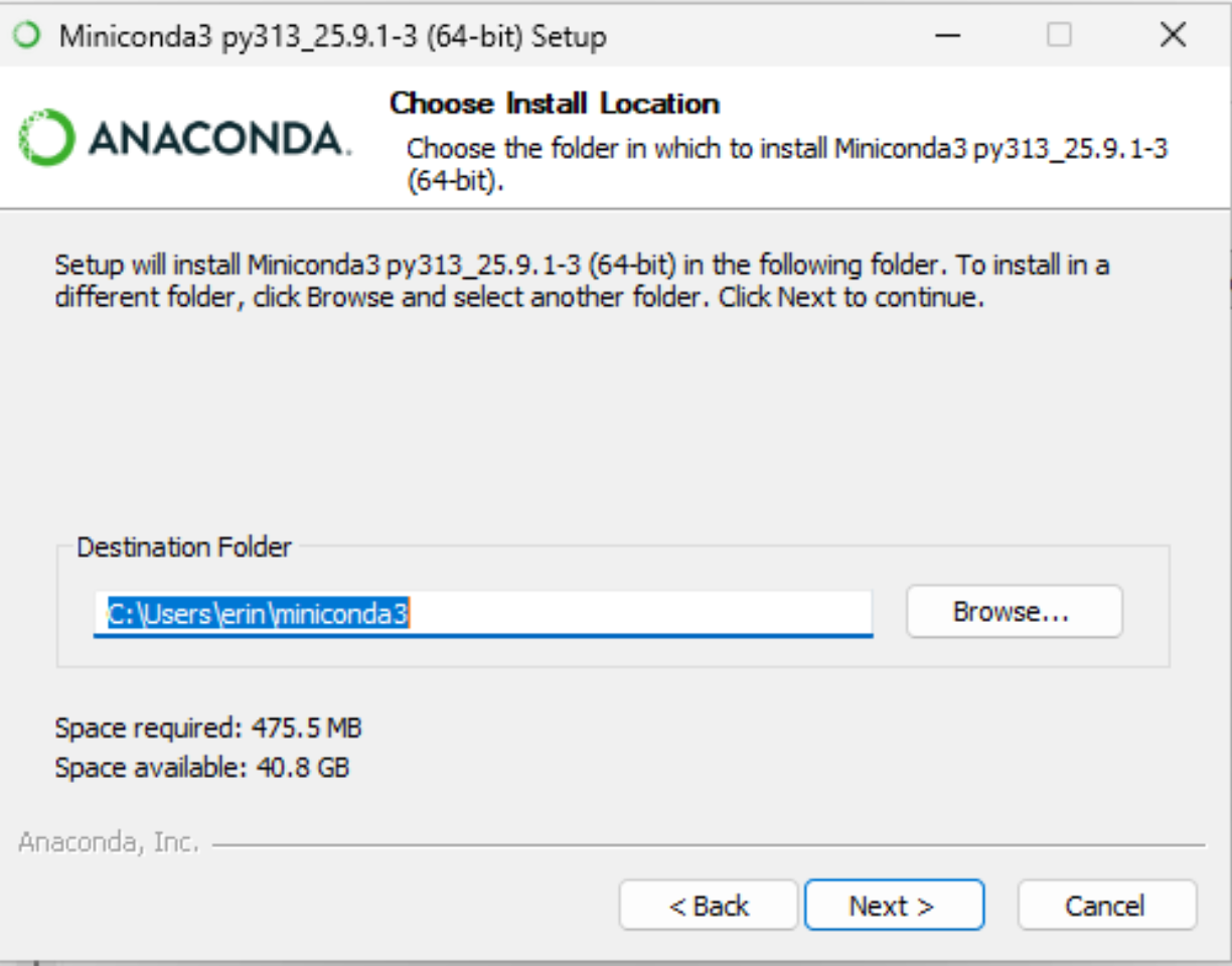
When asked about Advanced Installation Options make sure to check:
- Create shortcuts
- Register Miniconda3 as my default Python.
Leave the other boxes unchecked.
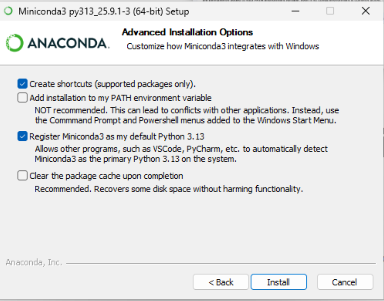
Click Install to install Miniconda. This should take less than five minutes.
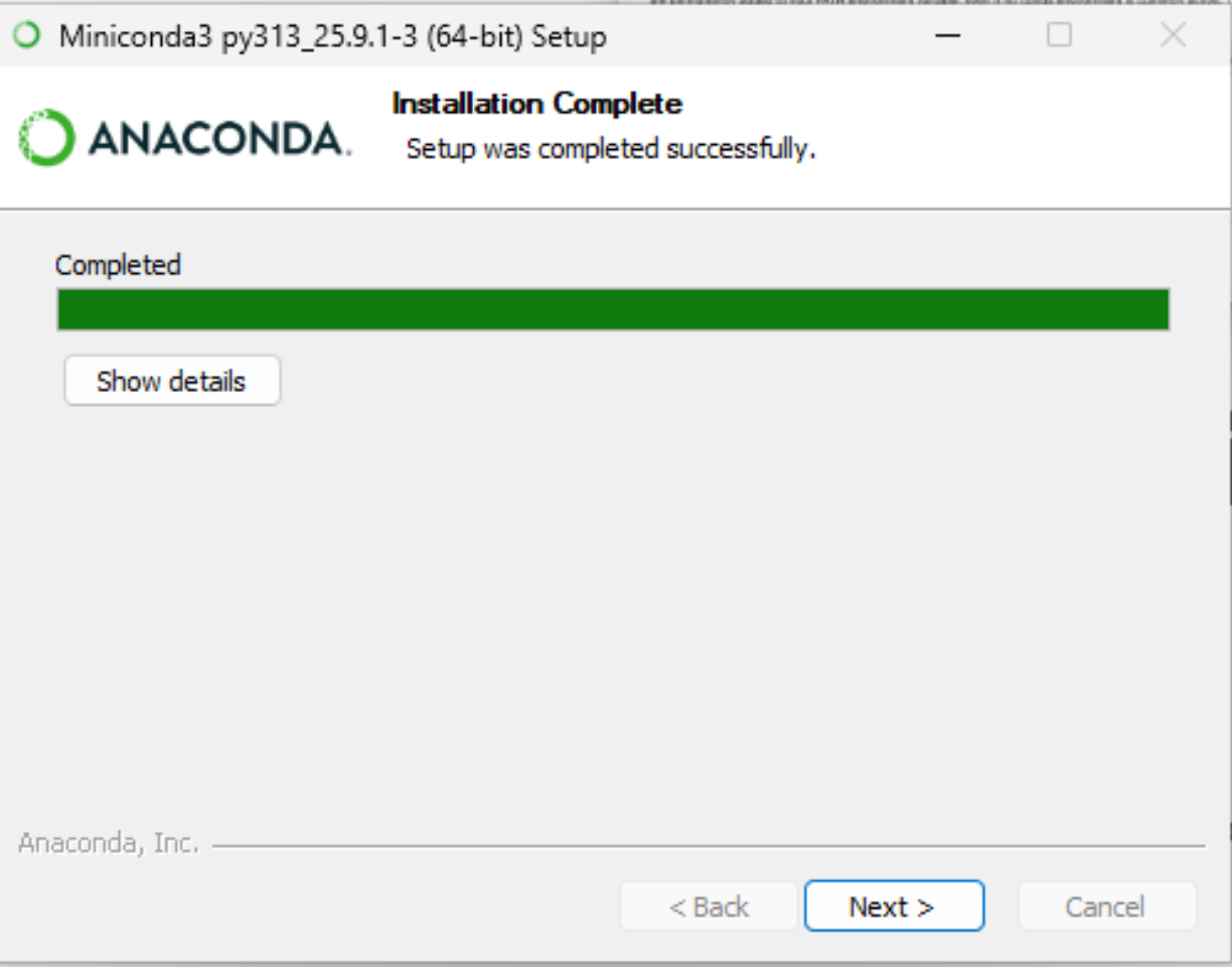
When the application has finished installing, click Next.
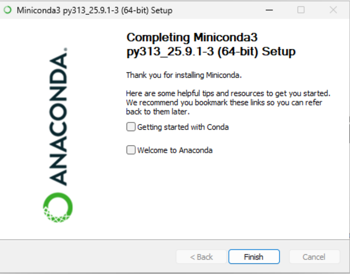
You will reach a final screen. Uncheck both boxes (you can read up on Miniconda later) and click Finish.
Installing JupyterLab
Click the symbol on the bottom of your screen or press the Windows ⊞ key on your keyboard. This will open up the Windows Start Menu.
In the Search box, type Anaconda Prompt. You should see a result like this:
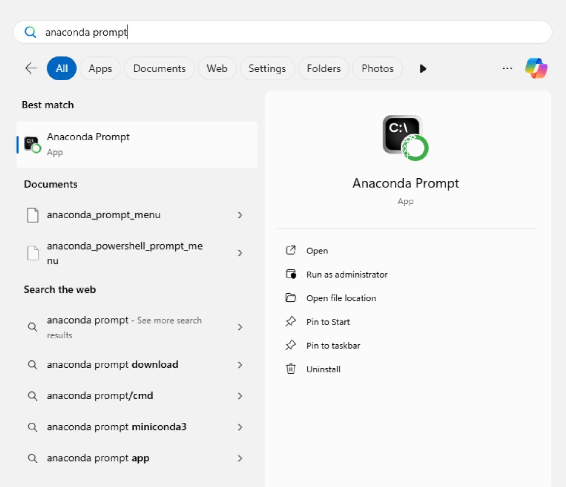
Click Pin to taskbar, as you’ll need this later.
Now, click on the Anaconda Prompt icon. A new window with a black screen will open.
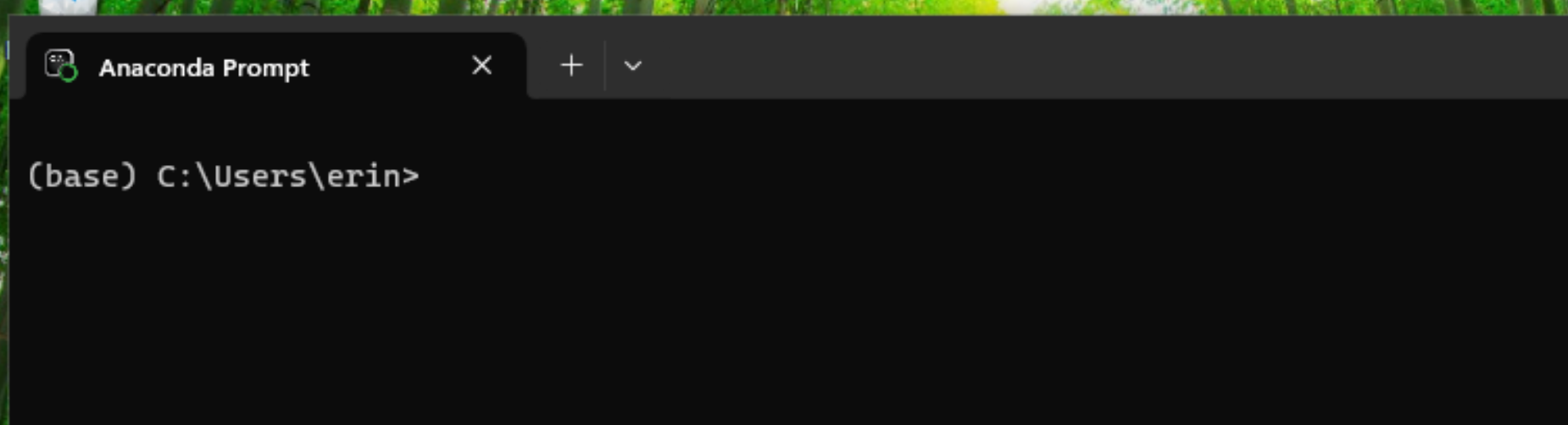
Inside the prompt window, type
conda install jupyterlab pandas matplotlib and press the
Enter key.
You may be prompted to press the a key twice, followed by the y key. The required software for this workshop will be downloaded from the internet.

After the installation finishes, you will see a message like the one above. Congratulations, you have installed Python and JupyterLab!
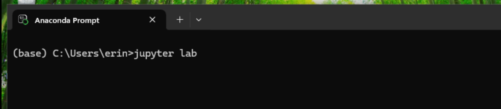
The JupyterLab Interface
JupyterLab has many features found in traditional integrated development environments (IDEs) but is focused on providing flexible building blocks for interactive, exploratory computing.
The JupyterLab Interface consists of the Menu Bar, a collapsible Left Side Bar, and the Main Work Area which contains tabs of documents and activities.
Menu Bar
The Menu Bar at the top of JupyterLab has the top-level menus that expose various actions available in JupyterLab along with their keyboard shortcuts (where applicable).
A screenshot of the default Menu Bar is provided below.

Main Work Area
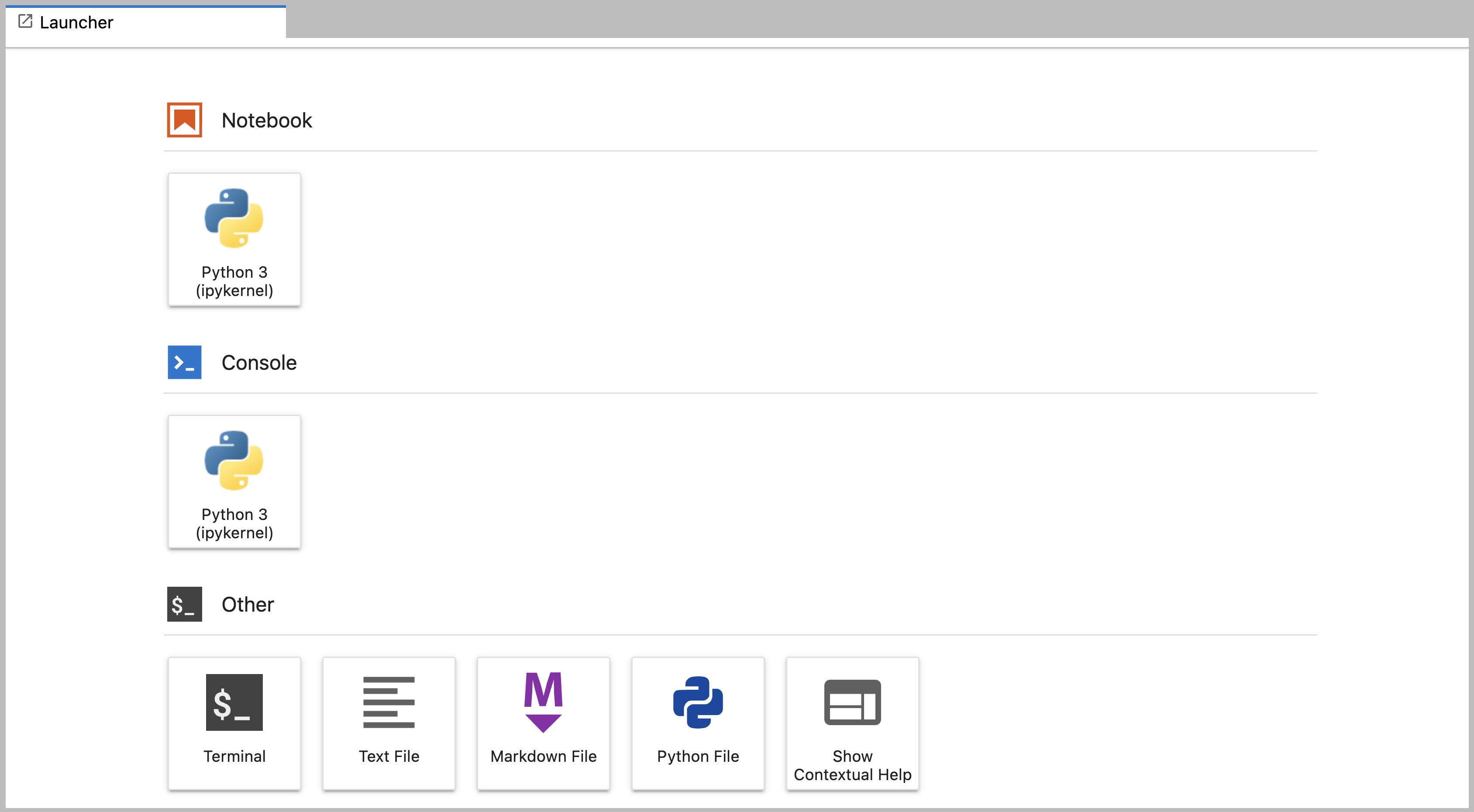
The main work area in JupyterLab enables you to arrange documents (notebooks, text files, etc.) and other activities (terminals, code consoles, etc.) into panels of tabs that can be resized or subdivided. A screenshot of the default Main Work Area is provided below.
If you do not see the Launcher tab, click the blue plus sign under the File and Edit menus and it will appear.
Left Sidebar
- By default, the left sidebar of a Jupyter notebook has a file browser showing the contents of the folder where JupyterLab was launched.
The directory where the JupyterLab server was launched will function as your working directory. This matters because if you want to reference other data files in your code, JupyterLab will look for them here by default. A screenshot of the default Left Side Bar is provided below.
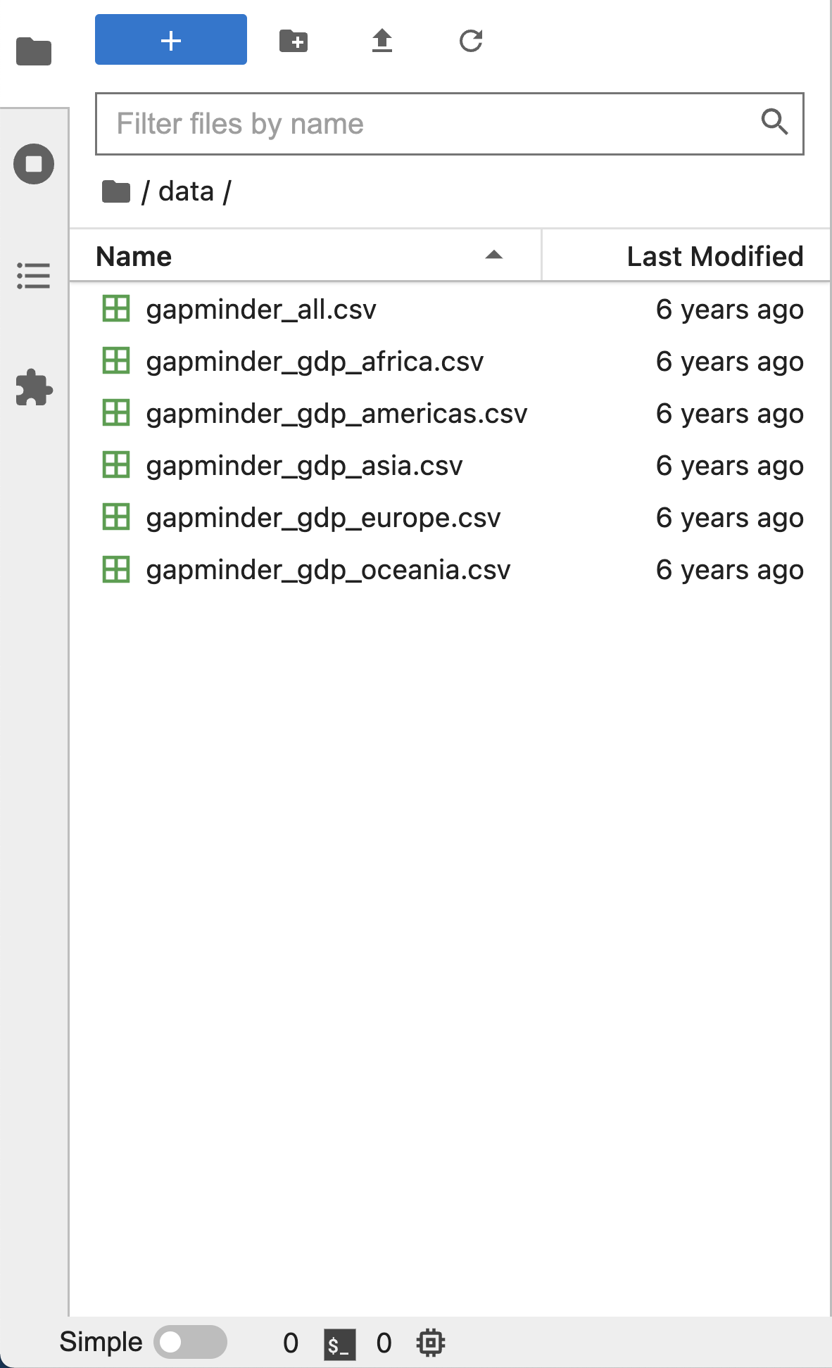
The left sidebar can be collapsed or expanded by selecting “Show Left Sidebar” in the View menu or by clicking on the active sidebar tab.
- Click on view in the menu bar. This opens a drop down menu of
options. Select “File Browser”
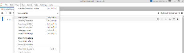
- When you click on File Browser, this will open the file directory as shown above.
What is a Working Directory?
- The working directory is, unless you specify otherwise, the location on your computer’s filesystem where Python will look for files you want to load and where it will put any files you save.
- You will write your code in Jupyter Notebooks, and save them later in a folder.
- It’s a good idea to save your data files in a named subfolder,
separate from your code. In this workshop your data files will be in
.csvformat.
Create a Folder for This Workshop
When you run the command jupyter lab in Terminal (MacOS)
or Anaconda Prompt (Windows), JupyterLab will launch in your home
directory.
Inside your Documents or Desktop folder, create a new folder named PythonWorkshop.
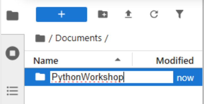
- First, click on your Documents folder in the File Browser on the
left.
- You should now see the contents of your Documents or My Documents folder.
- Next to the blue plus button at the top left of the File Browser,
you will see a folder icon.
- Click the New Folder icon.
- Name your new folder PythonWorkshop.
Navigate to that folder in the JupyterLab File Browser by clicking on it. You will use this folder in all future workshop sessions.
Create and Save a Jupyter Notebook File to your Working Directory
In the central pane of the JupyterLab interface, click on Python 3 in the Launcher to create a new Jupyter Notebook:
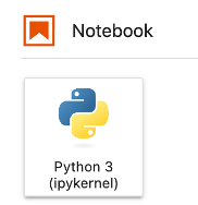
Use the menu or save icon to save this blank notebook. Make sure to
name it something helpful. For example, PythonWorkshop_1 or
PythonDay1. Notice that JupyterLab will append
.ipynb to the end of the name of the notebook. This is the
file extension for Jupyter Notebooks.
In the future, you can open your notebooks by navigating to the PythonWorkshop folder through the File Browser pane in JupyterLab.
You can see (and modify) this folder in File Explorer (Windows) or Finder (MacOS) too. Note that you cannot open your Python notebooks (.ipynb) by clicking on them from File Explorer or Finder. You must open them through the JupyterLab File Browser.
Verify your Working Directory
You can verify that you have the correct working directory by using what’s called a magic command.
Use the %pwd magic command within a code cell to print
the current working directory. The output will display the current
directory path.
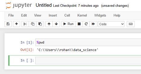
This magic command passes the “print working directory” command to your computer. Learn more about pwd here.
Your working directory path should end with
PythonWorkshop, the name of your project directory for this
workshop.
Key Points
- JupyterLab is an application for running, managing, and organizing Python code in files called Jupyter notebooks.
- You will only need to install JupyterLab once for this workshop.
- Your working directory determines where programs are run and how filepaths are interpreted.
Content from Running and Quitting
Last updated on 2026-10-05 | Edit this page
Overview
Questions
- How can I run Python programs?
Objectives
- Launch JupyterLab.
- Create a Jupyter notebook.
- Shut down the JupyterLab server.
- Create Markdown cells in a notebook.
- Create and run Python cells in a notebook.
- Distinguish between Markdown cells and Python cells.
Getting Started with JupyterLab
We’re going to use JupyterLab for the remainder of this workshop.
JupyterLab has several useful features for Python programmers:
- You can easily type, edit, and copy/paste blocks of code.
- Tab complete allows you to easily access the names of things you are using and learn more about them.
- You can annotate your code with links, different sized text, bullets, etc. to make it more accessible to you and your collaborators.
- It allows you to display visualizations next to the code that produces them to tell stories about data.
Starting JupyterLab
You can start the JupyterLab server through the command line via the
Terminal (Mac) or via Anaconda Prompt (Windows). Anaconda
Prompt is included as part of the Miniconda Python distribution you have
installed.
You cannot open Jupyter notebooks (.ipynb files) by
clicking on them directly. Instead, you will need to open JupyterLab and
open your notebooks using the JupyterLab File Browser.
macOS - Command Line
To start the JupyterLab server you will need to access the command line through the Terminal.
There are two ways to open Terminal on Mac.
- In your Applications folder, open Utilities and double-click on Terminal
- Press Command + spacebar to launch Spotlight.
Type
Terminaland then double-click the search result or hit Enter
Inside the Terminal, enter the following command to launch JupyterLab.
The JupyterLab Interface
JupyterLab has many features found in traditional integrated development environments (IDEs) but is focused on providing flexible building blocks for interactive, exploratory computing.
The JupyterLab Interface consists of the Menu Bar, a collapsable Left Side Bar, and the Main Work Area which contains tabs of documents and activities.
Menu Bar
The Menu Bar at the top of JupyterLab has the top-level menus that expose various actions available in JupyterLab along with their keyboard shortcuts (where applicable). The following menus are included by default.
- File: Actions related to files and directories such as New, Open, Close, Save, etc. The File menu also includes the Shut Down action used to shutdown the JupyterLab server.
- Edit: Actions related to editing documents and other activities such as Undo, Cut, Copy, Paste, etc.
- View: Actions that alter the appearance of JupyterLab.
- Run: Actions for running code.
- Kernel: Actions for managing kernels. Kernels in Jupyter will be explained in more detail below.
- Tabs: A list of the open documents and activities in the main work area.
- Settings: Common JupyterLab settings can be configured using this menu. There is also an Advanced Settings Editor option in the dropdown menu that provides more fine-grained control of JupyterLab settings and configuration options.
- Help: A list of JupyterLab and kernel help links.
Kernels
The JupyterLab docs define kernels as “separate processes started by the server that run your code in different programming languages and environments.”
- Opening a Jupyter Notebook starts a kernel process for running code.
- By default, Jupyter runs Python code using an IPython kernel.
- Using other Jupyter kernels for other programming languages would let us run code in other programming languages—like R, Julia, or Ruby—in the same JupyterLab interface.
A screenshot of the default Menu Bar is provided below.
Left Sidebar
The left sidebar contains a number of commonly used tabs, such as a file browser (showing the contents of the directory where the JupyterLab server was launched), a list of running kernels and terminals, the command palette, and a list of open tabs in the main work area. A screenshot of the default Left Side Bar is provided below.
The left sidebar can be collapsed or expanded by selecting “Show Left Sidebar” in the View menu or by clicking on the active sidebar tab.
Main Work Area
The main work area in JupyterLab enables you to arrange documents (notebooks, text files, etc.) and other activities (terminals, code consoles, etc.) into panels of tabs that can be resized or subdivided. A screenshot of the default Main Work Area is provided below.
If you do not see the Launcher tab, click the blue plus sign under the “File” and “Edit” menus and it will appear.
Drag a tab to the center of a tab panel to move the tab to the panel. Subdivide a tab panel by dragging a tab to the left, right, top, or bottom of the panel. The work area has a single current activity. The tab for the current activity is marked with a colored top border (blue by default).
Creating a Jupyter Notebook
To open a new notebook click the Python 3 icon under the Notebook header in the Launcher tab in the main work area. You can also create a new notebook by selecting New -> Notebook from the File menu in the Menu Bar.
Additional notes on Jupyter notebooks.
- Notebook files have the extension
.ipynbto distinguish them from plain-text Python programs. - Notebooks can be exported as Python scripts that can be run from the command line.
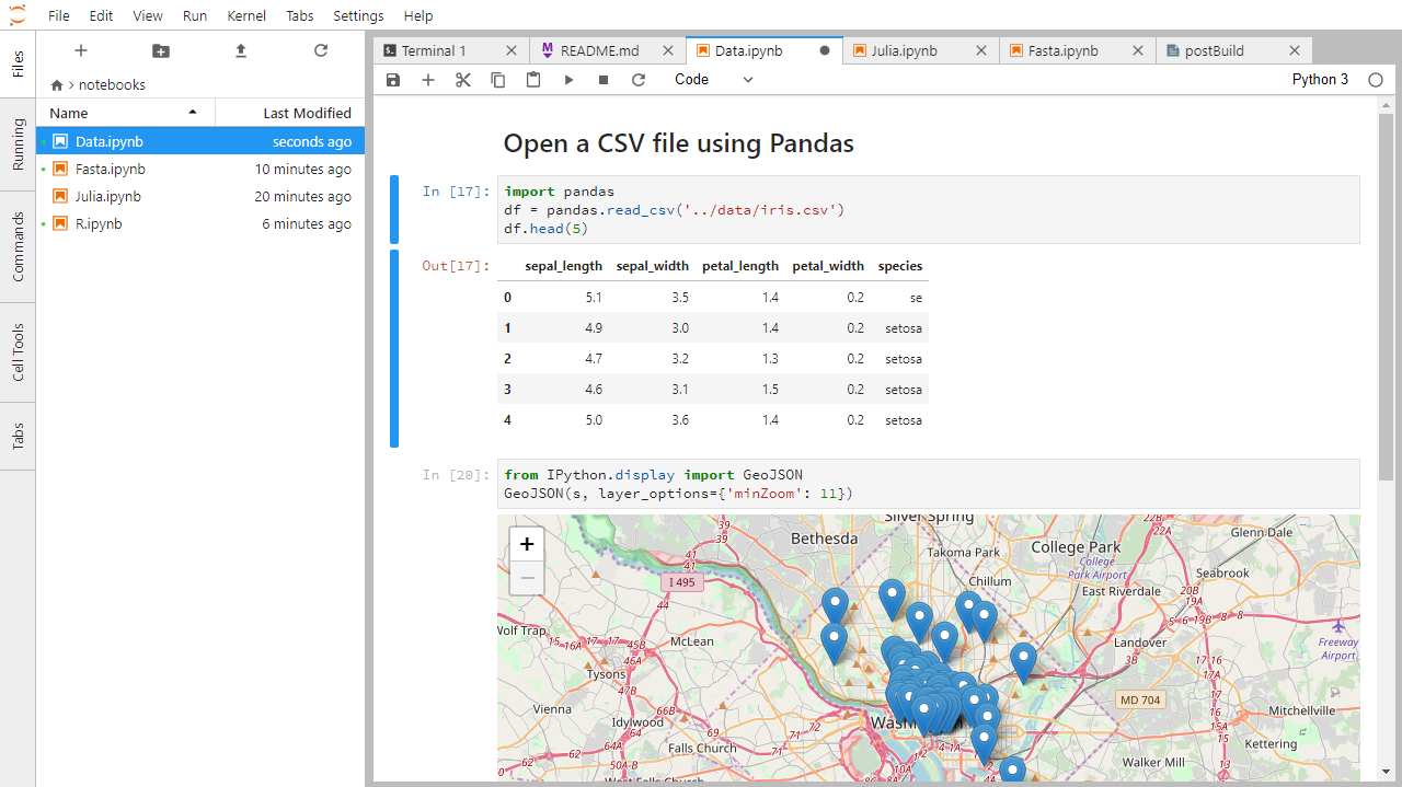
Below is a screenshot of a Jupyter notebook running inside JupyterLab. If you are interested in more details, then see the official notebook documentation.
How It’s Stored
- The notebook file is stored in a format called JSON.
- Just like a web page, what’s saved looks different from what you see in your browser.
- The JSON format allows Jupyter to mix source code, text, and images in one file.
Arranging Documents into Panels of Tabs
In the JupyterLab Main Work Area you can arrange documents into panels of tabs. Here is an example from the official documentation.
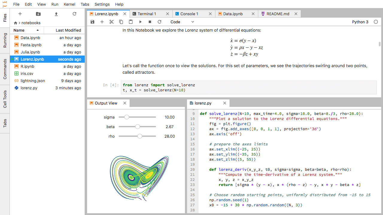
Use the Launcher to create a new text file called README.txt. Open your notebook, File Browser tab, and text file and arrange them into three panels in the main work area. What combination of panels and tabs do you think will be most useful for your workflow?
After creating the necessary tabs, you can drag one of the tabs to the center of a panel to move the tab to the panel; next you can subdivide a tab panel by dragging a tab to the left, right, top, or bottom of the panel.
Code vs. Text
Jupyter mixes code and text in different types of blocks, called cells. We use the term “code” to mean “code written in a language like Python.”
- In this class, a “code cell” will always contain Python.
- A “text cell” is one that contains ordinary prose written for human beings.
Using Python as a Calculator
Python can be used as a calculator to perform basic mathematical operations like multiplication and addition.

Create a new cell in your Jupyter notebook. Make sure it is a “Code” cell. Type the following and press the ▶ Play Button or Shift+Enter on your keyboard to run your code.
OUTPUT
8Python “knows” order of operations, so multiplication is applied before addition. Run the following calculation in a new cell.
OUTPUT
23Negative Numbers?
You can use parentheses with mathematical expressions in Python. Statements inside parentheses are always evaluated first.
Adjust the following code by inserting parentheses so that it returns a negative number as a result. Do not change anything else about the code.
Remember to run the code cell to check your work.
The Notebook has Command and Edit modes.
- If you press Esc and Return alternately, the outer border of your code cell will change from gray to blue.
- These are the Command (gray) and Edit (blue) modes of your notebook.
- Command mode allows you to edit notebook-level features, and Edit mode changes the content of cells.
- When in Command mode (esc/gray),
- The b key will make a new cell below the currently selected cell.
- The a key will make one above.
- The x key will delete the current cell.
- The z key will undo your last cell operation (which could be a deletion, creation, etc).
- All actions can be done using the menus, but there are lots of keyboard shortcuts to speed things up.
Command vs. Edit
- In the Jupyter notebook page are you currently in Command or Edit
mode?
- Switch between the modes.
- Use the shortcuts to generate a new cell.
- Use the shortcuts to delete a cell.
- Use the shortcuts to undo the last cell operation you performed.
Command mode has a gray border and Edit mode has a blue border. Use Esc and Return to switch between modes. You need to be in Command mode (Press Esc if your cell is blue). Type b or a. You need to be in Command mode (Press Esc if your cell is blue). Type x. You need to be in Command mode (Press Esc if your cell is blue). Type z.
Use the keyboard and mouse to select and edit cells.
- Pressing the Return key turns the border blue and engages Edit mode, which allows you to type within the cell.
- Because we want to be able to write many lines of code in a single cell, pressing the Return key when in Edit mode (blue) moves the cursor to the next line in the cell just like in a text editor.
- We need some other way to tell the Notebook we want to run what’s in the cell.
- Pressing Shift+Return together will execute the contents of the cell.
- Notice that the Return and Shift keys on the right of the keyboard are right next to each other.
The Notebook will turn Markdown into pretty-printed documentation.
- Notebooks can also render Markdown.
- A simple plain-text format for writing lists, links, and other things that might go into a web page.
- Equivalently, a subset of HTML that looks like what you’d send in an old-fashioned email.
- Turn the current cell into a Markdown cell by entering the Command mode (Esc/gray) and pressing the M key.
-
In [ ]:will disappear to show it is no longer a code cell and you will be able to write in Markdown. - Turn the current cell into a Code cell by entering the Command mode (Esc/gray) and pressing the y key.
Markdown allows you to “style” text cells.
Markdown code |
Rendered output |
|
|
|
|
| <p></p> | 1. Use numbers | 1. Use numbers | 1. to create | 2. to create | 1. numbered lists. | 3. numbered lists.
| | |
||
|
A Level-1 Heading |
|
|
A Level-2 Heading (etc.) |
|
|
Line breaks don’t matter. But blank lines create new paragraphs. |
|
|
Links | are created with
|
|
Adding Data to Your Project Folder
The data we will be using for this workshop is taken from the gapminder dataset.
To add the data to your Python project, download and unzip
the file python-novice-gapminder-data.zip
to your PythonWorkshop folder.
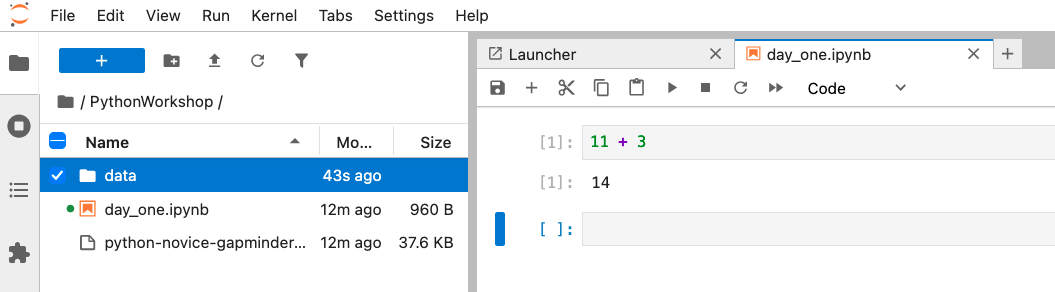
Double-click the zip file (MacOS) or right-click->Extract
All (Windows) to extract a folder of data. The unzipped folder will
be named data.
Copy the data folder into your
PythonWorkshop folder.
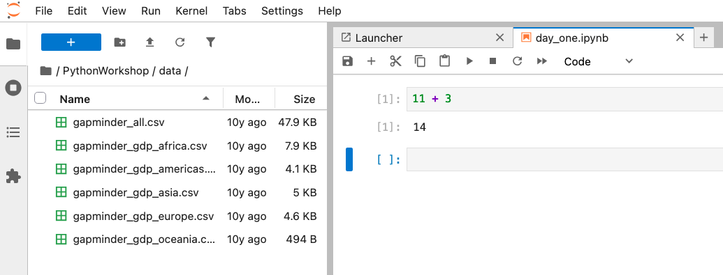
Click the ⟳ refresh symbol in the JupyterLab File Browser, then click
inside the data folder to inspect its contents from within
JupyterLab. You should see six files inside the data
folder.
Make sure you have a PythonWorkshop folder with a
data folder inside before the first workshop session
ends.
Closing JupyterLab
From the Menu Bar select the File menu and then choose Shut Down at the bottom of the dropdown menu. You will be prompted to confirm that you wish to shutdown the JupyterLab server (don’t forget to save your work!).
Click Shut Down to shut down the JupyterLab server.
You can now close the terminal application you used to launch the server.
To restart the JupyterLab server you will need to re-run the following command from Terminal (MacOS) or Anaconda Prompt (Windows).
Creating Lists in Markdown
Create a list in a Markdown cell in a notebook that looks like this:
- Get funding.
- Do work.
- Write up.
- Publish.
Your list should look like this.
1.  Get funding.
2.  Do work.
3.  Write up.
4. Publish.Change an Existing Cell from Code to Markdown
What happens if you write some Python in a code cell and then you switch it to a Markdown cell? For example, put the following in a code cell:
And then run it with Shift+Return to be sure that it works as a code cell. Now go back to the cell and use Esc then m to switch the cell to Markdown and “run” it with Shift+Return. What happened and how might this be useful?
Reasoning with True and False
Python can evaluate whether or not mathematical statements are True or False.
You can read the following statement as asking “is 3 less than 5?” Try running it.
OUTPUT
TrueChange one symbol in the following statement to make it
return True instead. Keep in mind that arithmetic is always
evaluated before operators like < or
>.
Key Points
- Use the JupyterLab Notebook interface for editing and running Python.
- Use the keyboard and mouse to select and edit cells.
- Jupyter Notebooks turn Markdown into pretty-printed documentation.
- Markdown can be used to format commentary on Python code.
Content from Variables and Assignment
Last updated on 2026-10-07 | Edit this page
Overview
Questions
- What basic data types can I work with in Python?
- How can I create a new variable in Python?
- How do I use the
print()function? - Can I change the value associated with a variable after I create it?
Objectives
- Write programs that assign values to variables.
- Correctly trace value changes in programs.
Variables
To do anything useful with data, we need to assign its value to a
variable. We assign a value
to a variable, using the equals
sign =.
For example, we can track the height of a patient by assigning the
value 65 to a variable height_cm:
In the future, Python will substitute the value we assigned to
height_cm when evaluating statements.
OUTPUT
65In Python, variable names:
- can include letters, digits, and underscores
- cannot start with a digit
- are case sensitive.
This means that, for example:
-
height0is a valid variable name, whereas0heightis not -
heightandheightare different variables
A variable is created when a value is assigned to it.
Here, Python assigns 42 to the variable age and a
string (always in quotes) to the variable
first_name.
Use print to display values.
- Python has a built-in function called
printthat prints things as text. - Call the function (i.e., tell Python to run it) by using its name.
- Provide values to the function (i.e., the things to print) in parentheses.
We can print a single value like this.
OUTPUT
65We can display multiple values in one line of output by passing in
comma-separated arguments to print().
OUTPUT
Ahmed is 42 years oldBy default, print function puts a single space between
items to separate them and wrapss them in a single line.
Variables must be created before they are used.
- If a variable doesn’t exist yet, or if the name has been mis-spelled, Python reports an error. (Unlike some languages, which “guess” a default value.)
ERROR
---------------------------------------------------------------------------
NameError                                 Traceback (most recent call last)
<ipython-input-1-c1fbb4e96102> in <module>()
----> 1 print(last_name)

NameError: name 'last_name' is not definedVariables Persist Between Cells
Be aware that it is the order of execution of cells that is important in a Jupyter notebook, not the order in which they appear. Python remembers all the code that was run previously in a given session, including any variables you have defined, irrespective of the order in the notebook.
If you define variables lower down the notebook and then (re)run cells further up, those defined further down will still be present. As an example, create two cells with the following content, in this order:
- If you execute this in order, the first cell will give an error.
- However, if you run the first cell after the second cell it
will print out
1. - To prevent confusion, it can be helpful to use the
Kernel->Restart & Run Alloption which restarts the kernel and runs everything from top to bottom. - A good Jupyter Notebook will execute as intended when cells are run from top to bottom.
Variables can be used in calculations.
We can use variables in calculations just as if they were values.
OUTPUT
Age in three years: 45Python is case-sensitive.
- Python thinks that upper- and lower-case letters are different, so
Nameandnameare different variables. - There are conventions for using upper-case letters at the start of variable names so we will use lower-case letters for now.
Use meaningful variable names.
- Python doesn’t care what you call variables as long as they obey the rules (alphanumeric characters and the underscore).
- Use meaningful variable names to help other people understand what the program does.
- The most important “other person” is your future self.
-
massholds a value of 47.5,agedoes not exist -
massstill holds a value of 47.5,ageholds a value of 122 -
massnow has a value of 95.0,age’s value is still 122 -
massstill has a value of 95.0,agenow holds 102
To prove this, print mass and age.
OUTPUT
mass is 95.0 age is 102Key Points
- Use variables to store values.
- Use
printto display values. - Variables persist between cells.
- Variables must be created before they are used.
- Variables can be used in calculations.
- Python is case-sensitive.
- Use meaningful variable names.
Content from Data Types and Type Conversion
Last updated on 2026-10-11 | Edit this page
Overview
Questions
- What kinds of data do programs store?
- How can I convert one type to another?
Objectives
- Explain key differences between integers and floating point numbers.
- Explain key differences between numbers and character strings.
- Use built-in functions to convert between integers, floating point numbers, and strings.
Every value has a type.
Every value in a program has a specific type.
We’re going to start with three basic data types in Python:
Use the built-in function type to find the type of a
value.
Use the built-in function type to find out what type a
value or variables has. Remember, the value has the type and
the variable is just a label.
OUTPUT
<class 'int'>OUTPUT
<class 'str'>Data types control what operations can be performed on a given value.
A value’s type determines what the program can do to it.
OUTPUT
2ERROR
---------------------------------------------------------------------------
TypeError                                 Traceback (most recent call last)
<ipython-input-2-67f5626a1e07> in <module>()
----> 1 print('hello' - 'h')

TypeError: unsupported operand type(s) for -: 'str' and 'str'
You can use the “+” and “*” operators on strings.
- “Adding” character strings concatenates them.
OUTPUT
Ahmed WalshMultiplying a character string by an integer N creates a new string that consists of that character string repeated N times because multiplication is repeated addition.
OUTPUT
==========Strings have a length (but numbers don’t).
The built-in function len counts the number of
characters in a string.
OUTPUT
3But numbers don’t have a length.
ERROR
---------------------------------------------------------------------------
TypeError                                 Traceback (most recent call last)
<ipython-input-3-f769e8e8097d> in <module>()
----> 1 print(len(52))

TypeError: object of type 'int' has no len()
You Must Convert Numbers to Strings and Vice-Versa to Use Them Together
You cannot add numbers and strings.
ERROR
---------------------------------------------------------------------------
TypeError                                 Traceback (most recent call last)
<ipython-input-4-fe4f54a023c6> in <module>()
----> 1 print(1 + '2')

TypeError: unsupported operand type(s) for +: 'int' and 'str'
This is not allowed because it’s ambiguous: should
1 + '2' be 3 or '12'?
Some types can be converted to other types by using the type name as a function.
OUTPUT
3
12
Can mix integers and floats freely in operations.
Integers and floating-point numbers can be mixed in arithmetic.
OUTPUT
half is 0.5
three squared is 9.0Automatic Type Conversion
What type of value is 3.25 + 4?
Use an index to get a character from a string.
- The characters (individual letters, numbers, and so on) in a string
are ordered. For example, the string
'AB'is not the same as'BA'. Because of this ordering, we can treat the string as a list of characters. - Each position in the string (first, second, etc.) is given a number. This number is called an index.
- Indices are numbered starting from 0.
- Use the position’s index in square brackets to get the character at that position.

OUTPUT
hUse a slice to get a substring.
- A part of a string is called a substring. A substring can be as short as a single character.
- A slice is a part of a string (or, more generally, a part of any list-like thing).
- We take a slice with the notation
[start:stop], wherestartis the integer index of the first element we want andstopis the integer index of the element just after the last element we want. - Taking a slice does not change the contents of the original string. Slicing returns a copy of part of the original string.
OUTPUT
sodUse the built-in function len to find the length of a
string.
OUTPUT
6Nested functions are evaluated from the inside out, like in mathematics.
Challenge
If you assign a = 123, what happens if you try to get
the second digit of a via a[1]?
OUTPUT
atom_name[1:3] is: arVariables change when something is assigned to them
OUTPUT
first is 2 and second is 5- Python reads the value of
v1when doing the multiplication, creates a new value, and assigns it tov2. - Afterwards, the value of
v1is set to the new value and not dependent onvariable_oneso its value does not automatically change whenv2changes.
Fractions
What type of value is 3.4? How can you find out?
Choose a Type
What type of value (integer, floating point number, or character string) would you use to represent each of the following? Try to come up with more than one good answer for each problem. For example, in # 1, when would counting days with a floating point variable make more sense than using an integer?
- Number of days since the start of the year.
- Serial number of a piece of lab equipment.
- Current population of a city.
- Average height of a group of students.
The answers to the questions are:
- Integer, since the number of days would lie between 1 and 365.
- A string because a serial number typically contains letters and numbers.
- I would use an integer to represent population in units of individuals.
- Floating point number, since an average is likely to have a fractional part.
Division Types
In Python 3, the // operator performs integer
(whole-number) floor division, the / operator performs
floating-point division, and the % (or modulo)
operator calculates and returns the remainder from integer division:
OUTPUT
5 // 3: 1
5 / 3: 1.6666666666666667
5 % 3: 2
Decide between the division types above for the following questions, then compute the answers in Python.
- The number of whole weeks per year given 365 days per year and 7 days per week.
- The average number of people per park in Eugene, OR given 179000 people and 135 parks.
- The number of leftover hats given 12 hats distributed evenly among 10 volunteers.
- This requires floor division, because you don’t care about partial weeks.
- This requires float division, because you want to preserve the decimal in an average.
- This requires the remainder, because you want the number of hats remaining after one hat is given out per person.
PYTHON
weeks_per_year = 365 // 7
people_per_park = 179000 / 135
leftover_hats = 12 % 10

print(weeks_per_year, people_per_park, leftover_hats)
OUTPUT
52 1325.9259259259259 2Strings to Numbers
Where reasonable, float() will convert a string to a
floating point number, and int() will convert a floating
point number to an integer:
OUTPUT
string to float: 3.4
float to int: 3
If the conversion doesn’t make sense, however, an error message will occur.
ERROR
---------------------------------------------------------------------------
ValueError                                Traceback (most recent call last)
<ipython-input-5-df3b790bf0a2> in <module>
----> 1 print("string to float:", float("Hello world!"))

ValueError: could not convert string to float: 'Hello world!'
Given this information, what do you expect the following program to do?
What does it actually do?
Why do you think it does that?
What do you expect this program to do? It would not be unreasonable
to expect the int command to convert the string “3.4” to
3.4.
OUTPUT
---------------------------------------------------------------------------
ValueError                                Traceback (most recent call last)
<ipython-input-2-ec6729dfccdc> in <module>
----> 1 int("3.4")
ValueError: invalid literal for int() with base 10: '3.4'
However, Python throws an error. Why? To be consistent, possibly. If you ask Python to perform two consecutive typecasts, you must convert it explicitly in code.
OUTPUT
3Arithmetic with Different Types
Answer: 1 and 4
Slicing concepts
Given the following string:
What would these expressions return?
species_name[2:8]-
species_name[11:](without a value after the colon) -
species_name[:4](without a value before the colon) -
species_name[:](just a colon) species_name[11:-3]species_name[-5:-3]- What happens when you choose a
stopvalue which is out of range? (i.e., tryspecies_name[0:20]orspecies_name[:103])
-
species_name[2:8]returns the substring'acia b' -
species_name[11:]returns the substring'folia', from position 11 until the end -
species_name[:4]returns the substring'Acac', from the start up to but not including position 4 -
species_name[:]returns the entire string'Acacia buxifolia' -
species_name[11:-3]returns the substring'fo', from the 11th position to the third last position -
species_name[-5:-3]also returns the substring'fo', from the fifth last position to the third last - If a part of the slice is out of range, the operation does not fail.
species_name[0:20]gives the same result asspecies_name[0:], andspecies_name[:103]gives the same result asspecies_name[:]
Key Points
- Every value has a type.
- Use the built-in function
typeto find the type of a value. - Types control what operations can be done on values.
- Strings can be added and mulitiplied.
- Strings have a length (but numbers don’t).
- Use an index to get a single character from a string.
- Use a slice to get a substring.
- Use the built-in function
lento find the length of a string. - Must convert numbers to strings or vice versa when operating on them.
- Can mix integers and floats freely in operations.
- Variables only change value when something is assigned to them.
Content from Built-in Functions and Help
Last updated on 2026-10-11 | Edit this page
Overview
Questions
- How can I use built-in functions?
- How can I find out what they do?
- What kind of errors can occur in programs?
Objectives
- Explain the purpose of functions.
- Correctly call built-in Python functions.
- Correctly nest calls to built-in functions.
- Use help to display documentation for built-in functions.
- Describe (and correct) situations in which SyntaxError and NameError occur.
Use comments to add documentation to programs.
Python ignores lines that begin with the # symbol. Use
these to create comments to annotate your code.
PYTHON
# This sentence isn't executed by Python.
adjustment = 0.5   # Neither is this - anything after '#' is ignored.
Comments do not change how Python code behaves.
OUTPUT
0.5A function may take zero or more arguments.
We have seen some functions already: now, let’s take a closer look.
- An argument is a value passed into a function. Functions take 0 or more arguments.
-
lentakes exactly one. -
int,str, andfloatalso take one argument. -
printtakes zero or more. -
printwith no arguments prints a blank line.- Must always use parentheses, even if they’re empty, so that Python knows a function is being called.
OUTPUT
before

after
Every function returns something.
- Every function call produces some result.
- If the function doesn’t have a useful result to return, it usually
returns the special value
None.Noneis a Python object that stands in anytime there is no value.
OUTPUT
example
result of print is None
Commonly-used built-in functions include max,
min, and round.
- Use
maxto find the largest value of one or more values. - Use
minto find the smallest of one or more values. - These functions work on strings as well. Characters in strings are compared using ASCII values.
OUTPUT
3
0
Functions may only work for certain (combinations of) arguments.
-
maxandminmust be given at least one argument. - When given two or more arguments, they must be comparable.
ERROR
TypeError                                 Traceback (most recent call last)
<ipython-input-52-3f049acf3762> in <module>
----> 1 print(max(1, 'a'))

TypeError: '>' not supported between instances of 'str' and 'int'
Functions may have default values for some arguments.
The round function rounds off a floating-point number.
By default, it rounds to zero decimal places, ie. the nearest
integer.
OUTPUT
4You can specify the number of decimal places to round to as a second argument.
OUTPUT
3.7Use help to get help for a function.
How could you have known what the 1 in
round(3.712, 1) does if you hadn’t been told? When learning
new Python functions, you should read about them carefully.
You can use help() followed by the name of a function
(without parentheses) to get information about what a function does and
what arguments it expects.
OUTPUT
Help on built-in function round in module builtins:

round(number, ndigits=None)
    Round a number to a given precision in decimal digits.

    The return value is an integer if ndigits is omitted or None.
    Otherwise the return value has the same type as the number.  ndigits
    may be negative.
Functions attached to objects are called methods
Methods are special functions that come after an object, followed by
a . symbol. Methods are said to be bound to
objects of a particular type.
PYTHON
my_string = 'Hello world!'  # Create and assign my_string

print(len(my_string))       # the len function takes a string as an argument and returns the length of the string

print(my_string.swapcase()) # calling the swapcase method on the my_string object

print(my_string.__len__())  # calling the internal __len__ method on the my_string object, used by len(my_string)
OUTPUT
12
hELLO WORLD!
12
Methods (and functions) can be chained together. They always operate from left to right.
PYTHON
print(my_string.isupper())          # Not all the letters are uppercase
print(my_string.upper())            # This capitalizes all the letters

print(my_string.upper().isupper())  # Now all the letters are uppercase
OUTPUT
False
HELLO WORLD
True
The Jupyter Notebook has two ways to get help.
Option 1: Place the cursor near where the function is invoked in a cell (i.e., the function name or its parameters), - Hold down Shift, and press Tab. - Do this several times to expand the information returned. Option 2: Type the function name in a cell with a question mark after it. Then run the cell.
Python reports a syntax error when it can’t understand the source of a program.
Grammatically incorrect Python produces syntax errors. The most common syntax errors involve failure to close quotes, parentheses, or improper indentation.
ERROR
  File "<ipython-input-56-f42768451d55>", line 2
    name = 'Feng
                ^
SyntaxError: EOL while scanning string literalERROR
  File "<ipython-input-57-ccc3df3cf902>", line 2
    age = = 52
          ^
SyntaxError: invalid syntax
Look closely at error messages to figure out what to fix.
ERROR
  File "<ipython-input-6-d1cc229bf815>", line 1
    print ("hello world"
                        ^
SyntaxError: unexpected EOF while parsing
The message indicates a problem on first line of the input (“line
1”). - The -6- part of the filename indicates that the
error occurred in cell 6 of our Notebook. - Next is the problematic line
of code, indicating the problem with a ^ pointer.
Python reports a runtime error when something goes wrong while a program is executing.
ERROR
NameError                                 Traceback (most recent call last)
<ipython-input-59-1214fb6c55fc> in <module>
      1 age = 53
----> 2 remaining = 100 - aege # mis-spelled 'age'

NameError: name 'aege' is not defined- Fix syntax errors by reading the source and runtime errors by tracing execution.
Other ways to get help
There are several other ways that people often get help when they are stuck with their Python code.
- Search the internet: paste the last line of your error message or
the word “python” and a short description of what you want to do into
your favourite search engine and you will usually find several examples
where other people have encountered the same problem and came looking
for help.
- StackOverflow can be particularly helpful for this: answers to questions are presented as a ranked thread ordered according to how useful other users found them to be.
- Take care: copying and pasting code written by somebody else is risky unless you understand exactly what it is doing!
- Ask somebody “in the real world”. If you have a colleague or friend with more expertise in Python than you have, show them the problem you are having and ask them for help.
What About Generative AI?
We recommend against using generative AI tools for the exercises in this workshop. This workshop is intended to teach you the grammar of Python and strategies for solving programming problems. You will not be able to understand or evaluate the results of Generate AI tools, should you choose to use them, if you do not master the fundamental skills presented here.
What Happens When
- Order of operations:
1.1 * radiance = 1.11.1 - 0.5 = 0.6min(radiance, 0.6) = 0.62.0 + 0.6 = 2.6max(2.1, 2.6) = 2.6- At the end,
radiance = 2.6
Spot the Difference
- Predict what each of the
printstatements in the program below will print. - Does
max(len(rich), poor)run or produce an error message? If it runs, does its result make any sense?
OUTPUT
cOUTPUT
tinOUTPUT
4max(len(rich), poor) throws a TypeError. This turns into
max(4, 'tin') and as we discussed earlier a string and
integer cannot meaningfully be compared.
ERROR
TypeError                                 Traceback (most recent call last)
<ipython-input-65-bc82ad05177a> in <module>
----> 1 max(len(rich), poor)

TypeError: '>' not supported between instances of 'str' and 'int'Explore the Python docs!
The official Python documentation is arguably the most complete source of information about the language. It is available in different languages and contains a lot of useful resources. The Built-in Functions page contains a catalogue of all of these functions, including the ones that we’ve covered in this lesson. Some of these are more advanced and unnecessary at the moment, but others are very simple and useful.
Key Points
- Use comments to add documentation to programs.
- A function may take zero or more arguments.
- Commonly-used built-in functions include
max,min, andround. - Functions may only work for certain (combinations of) arguments.
- Functions may have default values for some arguments.
- Use the built-in function
helpto get help for a function. - The Jupyter Notebook has two ways to get help.
- Every function returns something.
- Python reports a syntax error when it can’t understand the source of a program.
- Python reports a runtime error when something goes wrong while a program is executing.
- Fix syntax errors by reading the source code, and runtime errors by tracing the program’s execution.
Content from Lists
Last updated on 2026-10-21 | Edit this page
Overview
Questions
- How can I store multiple values in one object.
Objectives
- Explain what a Python list is.
- Explain why programs need collections of values.
- Write programs that create lists, index them, slice them, and modify them.
Lists stores values of any type
A list stores multiple values in one object, in a specific order. Values in a list can be called “elements” or “items”.
A list is represented by comma-separated items enclosed in
[].
OUTPUT
['my', 'first', 'list']Items in a list do not have to be of the same type.
OUTPUT
['15', 31, 12.0]Use len to find out how many values are in a list.
OUTPUT
3Lists are indexed like strings
Just like strings, lists are indexed from 0 to n-1, where n is the length of the list. Use [] to select indexed values.
PYTHON
alphabet = "abcde"
words = ["apple", "boy", "camel", "dog"]

print(alphabet[1])
print(words[1])
OUTPUT
b
boy
Make sure you check the length of a list before indexing into it. As with strings, indexing into a value that doesn’t exist (because the list is too short) causes an IndexError.
OUTPUT
IndexError                                Traceback (most recent call last)
Cell In[80], line 1
----> 1 words[5]

IndexError: list index out of range
You can also use the same syntax [start:stop] you used
to express slices for strings with lists.
OUTPUT
['apple', 'boy']Values in lists can be reassigned
Use indexing on the left side of an assignment statement to replace a value inside a list.
Lists are mutable: they can be changed after they are instantiated.
PYTHON
pressures = [0.273, 0.275, 0.277, 0.275, 0.276]
pressures[0] = 0.26
print('Pressures is now:', pressures)
OUTPUT
pressures is now: [0.265, 0.275, 0.277, 0.275, 0.276]The append method adds items to the end of a list
Use the .append method to add items to the end of a
list.
PYTHON
primes = [2, 3, 5]
print('primes is initially:', primes)
primes.append(7)
print('primes has become:', primes)
OUTPUT
primes is initially: [2, 3, 5]
primes has become: [2, 3, 5, 7]
The .append() method returns None and modifies the list
in place. That is, it directly modifies the list that calls the method
rather than returning a copy.
This is an intentional design choice.
PYTHON
returned_by_append = primes.append(11) # Append 11 but return None
print(returned_by_append)
print(primes)
OUTPUT
None
[2, 3, 5, 7, 11]
Extending a list concatenates two lists together
Use the .extend() method to add a list passed in as an argument to the end of that list.
PYTHON
housemates = ["dave", "rose"]
guests = ["bob", "yao", "sam"]
guests.extend(housemates) # Also modifies in place
print("The following people will be at my party", guests)
print("There are", len(guests), "guests")
OUTPUT
The following people will be at my party ['bob', 'yao', 'sam', 'dave', 'rose']
There are 5 guests
Appending a list to a list creates a nested list: a list inside of a list.
OUTPUT
[1, 'dog', 'antelope', [2, 2, 3]]The empty list contains no values.
We don’t have to create lists with items already in them. The empty
list [] is a list with length 0.
OUTPUT
0You can think of it as “the zero of lists.”
The empty list is useful because we can add items to it using methods
like .append() and .extend().
OUTPUT
[4, 5]Inserting into list with .insert()
So far, we’ve looked at methods that modify the end of a list.
The method .insert(i, x) inserts item x
before the item at position i.
PYTHON
alpha = ["apple", "berry", "durian"]
alpha.insert(2, "cherry") # Before the item at index 2 ("durian")
print(alpha)
OUTPUT
['apple', 'berry', 'cherry', 'durian']Removing items from lists: del, .remove(), and .pop()
We use del list_name[index] to remove an element from a
list. - del is not a function or a method, but a statement
in the language.
PYTHON
primes = [2, 3, 5, 7, 9]
print('primes before removing', primes)
del primes[4]
print('primes after removing', primes)
OUTPUT
primes before removing: [2, 3, 5, 7, 9]
primes after removing: [2, 3, 5, 7]
However, it is more common to see items removed from lists using the
.remove() and .pop() methods.
.remove(x) will remove the first instance of value(x) from
a list. Like .append(), the .remove() function
returns None.
OUTPUT
['sam']It will return a ValueError if there are no instances of x in the
list. Now that “rose” has already moved out, .remove() will
fail because it cannot find a “rose” in the list to remove.
OUTPUT
----> 1 housemates.remove("rose")

ValueError: list.remove(x): x not in list
Let’s say two new housemates move in: “josh” and “joe”.
PYTHON
housemates.append("josh")
housemates.append("joe")
print("There are now", len(housemates), "people in the house.")
The landlord imposes a new rule. Only two people are allowed in the house. The person who moved in most recently (the end of the list) must move out.
We can use the .pop() method to remove (and return) the
last item in a list.
PYTHON
evicted = housemates.pop() # Removes and returns the last item in a list
print(evicted, "was evicted.")
print(housemates, "live in the house")outputjoe was evicted. ['sam', 'josh'] live in the house
You cannot .pop() values from an empty list.
OUTPUT
IndexError                                Traceback (most recent call last)
Cell In[23], line 2
      1 empty_house = []
----> 2 empty_house.pop()

IndexError: pop from empty list
Character strings are immutable.
We cannot change the characters in a string after it has been created because Python considers the string to be a single primitive value.
Primitives (strings, ints, floats, booleans) are immutable. This means that when we want to change the value of a string or number variable, we can only replace the old value with a completely new value.
ERROR
TypeError: 'str' object does not support item assignmentLists and character strings are both collections.
Mutable and immutable objects: when a copy isn’t a copy
Be careful when modifying data in-place. If two variables refer to the same list, and you modify the list value, it will change for both variables!
This has to do with the mechanics of assignment and mutability in Python.
OUTPUT
[1, 3, 5]
y [1, 3, 5] is another name for x
If you wish to make two copies of the same list, use the
.copy() method instead. This method returns a new list with
the same contents. This principle applies for all mutable
variables. (We’ll learn about another mutable data type—the
DataFrame—later in this workshop.)
PYTHON
x = [1, 3]
y = x.copy() # Y points to a different, mutable list
x.append(5)
print("x", x)
print("y", y, "hasn't changed.")
OUTPUT
x [1, 3, 5]
y [1, 3] hasn't changed.
For additional reading on this topic, see this question from the official Python FAQ.
Two ways of sorting lists
There are two common ways to sort lists by their values: the
sorted() function which returns a sorted collection as a
copy and the .sort() method which sorts a list in
place.
PYTHON
numbers = [1, 5, 3, 4, 2]
snumbers = sorted(numbers) # Returns a copy
print(numbers) # Unchanged
print(snumbers)
OUTPUT
[1, 5, 3, 4, 2]
[1, 2, 3, 4, 5]
Notice that the .sort() method returns None
and permanently changes numbers.
PYTHON
print("Numbers before .sort()", numbers)
numbers.sort() # Permanently changes numbers
print("Numbers after", numbers)
OUTPUT
Numbers before .sort() [1, 5, 3, 4, 2]
Numbers after [1, 2, 3, 4, 5]
However, sorting a list only works when all its values are of the
same data type. Remember those rules about comparing items of different
types with min() and max()?
OUTPUT
TypeError                                 Traceback (most recent call last)
Cell In[27], line 1
----> 1 valid_list.sort()

TypeError: '<' not supported between instances of 'int' and 'str'How Large is a Slice?
If start and stop are both non-negative
integers, how long is the list values[start:stop]?
The list values[start:stop] has up to
stop - start elements. For example,
values[1:4] has the 3 elements values[1],
values[2], and values[3]. Why ‘up to’? As we
saw in episode 2, if stop
is greater than the total length of the list values, we
will still get a list back but it will be shorter than expected.
-
list('some string')converts a string into a list containing all of its characters. -
joinreturns a string that is the concatenation of each string element in the list and adds the separator between each element in the list. This results inx-y-z. The separator between the elements is the string that provides this method.
Working With the End
What does the following program print?
- How does Python interpret a negative index?
- If a list or string has N elements, what is the most negative index that can safely be used with it, and what location does that index represent?
- If
valuesis a list, what doesdel values[-1]do? - How can you display all elements but the last one without changing
values? (Hint: you will need to combine slicing and negative indexing.)
The program prints m.
- Python interprets a negative index as starting from the end (as
opposed to starting from the beginning). The last element is
-1. - The last index that can safely be used with a list of N elements is
element
-N, which represents the first element. -
del values[-1]removes the last element from the list. values[:-1]
OUTPUT
lithiumThe first statement prints the whole string, since the slice goes beyond the total length of the string. The second statement returns an empty string, because the slice goes “out of bounds” of the string.
Program A prints
OUTPUT
letters is ['g', 'o', 'l', 'd'] and result is ['d', 'g', 'l', 'o']Program B prints
OUTPUT
letters is ['d', 'g', 'l', 'o'] and result is Nonesorted(letters) returns a sorted copy of the list
letters (the original list letters remains
unchanged), while letters.sort() sorts the list
letters in-place and does not return anything.
Key Points
- A list stores many values in a single structure.
- Use an item’s index to fetch it from a list.
- Lists’ values can be replaced by assigning to them.
- Appending items to a list lengthens it.
- Use
delto remove items from a list entirely. - The empty list contains no values.
- Lists may contain values of different types.
- Character strings can be indexed like lists.
- Character strings are immutable.
- Indexing beyond the end of the collection is an error.
Content from For Loops
Last updated on 2026-10-19 | Edit this page
Overview
Questions
- How can I make a program repeat things?
Objectives
- Explain what a for loop does.
- Correctly write for loops to repeat simple calculations.
- Trace changes to a loop variable as the loop runs.
- Trace changes to other variables as they are updated by a for loop.
The power of programming comes from repetition
So far, we’ve been looking manipulating one value at a time. To write programs that are useful for manipulating real data, we need to make Python perform repetitive tasks for us.
An example task that we might want to repeat is accessing numbers in a list. We could do this printing each number on a line of its own.
OUTPUT
1
3
5
7
This is a bad approach for three reasons:
- It’s not scalable. We’d have to write hundreds of
print()statements for a longer list. - It’s difficult to maintain.
- It’s fragile. What happens if a list is shorter than we expected? (An error.)
We can solve this problem using a for loop that steps through each item in a collection.
OUTPUT
1
3
5
7
A for loop executes commands once for each value in a collection.
A for loop tells Python to execute some statements once for each value in a list, a character string, or some other collection.
The loop has three parts: an iterable, a loop variable, and a body that is repeated once for each item in the iterable. The name of a loop variable can be any valid variable name.
Let’s anatomize this loop:
- The iterable,
[2, 3, 5], is what the loop is being run on. It is followed by a:. - The body,
print(number), specifies what to do for each value in the collection. - The loop variable,
number, is what changes for each iteration of the loop.
This for loop is equivalent to:
And the for loop’s output is:
OUTPUT
2
3
5
The first line of the for loop must end with a colon,
and the body must be indented.
The colon at the end of the first line signals the start of a block of statements. Any consistent indentation is grammatical, but almost everyone uses four spaces or the tab key.
ERROR
IndentationError: expected an indented blockPython is picky about indentation and will not parse unexpected indents.
ERROR
  File "<ipython-input-7-f65f2962bf9c>", line 2
    lastName = "Smith"
    ^
IndentationError: unexpected indentClassifying Errors
Is an indentation error a syntax error or a runtime error?
An IndentationError is a syntax error. Programs with syntax errors cannot be started. A program with a runtime error will start but an error will be thrown under certain conditions.
Loop variables can be called anything.
As with all variables, loop variables are: * Created on demand. * Can have any valid variable name.
OUTPUT
2
3
5The body of a loop can contain many statements.
The body of a loop can contain multiple statements, as long as they’re all indented appropriately. All indented lines (an indented block) before the first unintended line are treated as part of the same loop and are evaluated in order.
PYTHON
primes = [2, 3, 5] # First three primes
for p in primes:
    squared = p ** 2
    cubed = p ** 3
    print(p, squared, cubed)
OUTPUT
2 4 8
3 9 27
5 25 125This code has a common mistake: the iterable (squares) is used in
place of the loop variable. While raising a number to the
0.5 power is equivalent to applying the square root of a
number, you can’t get the square root of a list!
OUTPUT
1.0
2.0
3.0
4.0
The range() function iterates over a sequence of
numbers.
Use range() to iterate over a sequence of numbers.
- The built-in function range produces a sequence of numbers.
- Not a list: the numbers are produced on demand to make looping over large ranges more efficient.
-
range(N)is the numbers 0..N-1
OUTPUT
0
1
2
3
4
The range() function is convenient when you want to do
an operation a fixed number of times.
PYTHON
housemates = ["joe", "james", "yao"] # Iterated in order
for housemate in range(len(housemates)):
    name = housemates.pop()
    print(name, "moved out")
print(housemates)
OUTPUT
yao moved out
james moved out
joe moved out
[]
The numbers in a range can be adjusted by their start, stop, and step arguments. If a single integer is supplied, it is assumed to be the stop. The default value of step is 1, ie. it is incremented by 1.
PYTHON
one_to_five = range(1, 6) # Start at 1, stop before 6 (exclusive)
for num in one_to_five:
    print(num)
OUTPUT
1
2
3
4
5
Set the step parameter to -1 to have the range count down rather than up. The start is still inclusive and the stop is still exclusive.
PYTHON
five_to_one = range(5, 0, -1) # Start at 5 (inclusive), stop at 0 (exclusive), -1 to step
for num in five_to_one:
    print(num)
OUTPUT
5
4
3
2
1
Programming pattern: accumulation
A common pattern in programs is to:
- Initialize an accumulator variable to zero, the empty string, or the empty list.
- Update the variable with values from a collection
Let’s say we want to compute the sum of the first five integers
starting at 1. You will need to initalize a varable called
total to 0. This will be our accumulator variable.
PYTHON
# Sum the first 10 integers.
total = 0 # Initialize a variable called sum
for num in range(1, 6):
    print("Total", total)
    print("Adding", num)
    total = total + num # same as total += num
print(total)
OUTPUT
Total 0
Adding 1
Total 1
Adding 2
Total 3
Adding 3
Total 6
Adding 4
Total 10
Adding 5
15
Let’s find the total length (in characters) of the strings in the
following list: ["red", "green", "blue"].
OUTPUT
12Debugging Accumulators
Let’s say you want to compute the factorial of 6 or \(6!\) by hand. This is equal to 6 * 5 * 4 * 3 * 2 * 1. We can use a for-loop and an accumulator pattern to do this.
Let’s say your first draft looks like this.
PYTHON
accumulator = 0
for i in range(1, 7): # 1 inclusive to 7 exclusive
    print(i)
    accumulator = accumulator * i
print("6! = ", accumulator)
Is the answer correct? What needs to be changed about this block of code in order for it to compute \(6!\) correctly?
You’re multiplying rather than adding. Making your accumulator start at 0 will 0 out your results, as the product of any number * 0 is 0. Therefore, to get the correct result, you want \(1 * (6 * 5 * 4 * 3 * 2 * 1)\). Setting accumulator to 1 fixes this.s
Key Points
- A for loop executes commands once for each value in a collection.
- A for loop is made up of a collection, a loop variable, and a body.
- The first line of the for loop must end with a colon, and the body must be indented.
- Indentation is always meaningful in Python.
- Loop variables can be called anything (but it is strongly advised to have a meaningful name to the looping variable).
- The body of a loop can contain many statements.
- Use range() to iterate over a sequence of numbers.
Content from Conditionals
Last updated on 2026-10-21 | Edit this page
Overview
Questions
- How can my programs do different things based on data values?
Objectives
- Write conditional statements including if, elif, and else branches.
- Trace the execution of conditionals.
- Apply conditionals inside loops.
Booleans can be True or False
We’ve discussed the following primitive data types so far: strings, ints, and floats. Let’s add bools or Booleans to that list.
Booleans can be True or False. They are
returned by conditional statements formed with operators like
==, <, or >.
OUTPUT
FalseThe == sign and = have very different
meanings in Python. The == sign tests whether or not two
values are equal.
OUTPUT
TrueUse if statements to control whether or not a block of code is executed
Today, we will discuss control flow, one of the most powerful aspects of programming languages.
- An if statement controls whether or not a block of code is executed.
- The first line of an if statement starts with
ifand ends with a colon. - The body of an if statement is indented, just like a for loop.
PYTHON
temp_f = 95
if temp_f > 90: # The indented block runs if (temp_f > 90) is True
    print("Specimen is too hot")
OUTPUT
Specimen is too hotIf the condition tested in the if statement evalutates to
True, then the block of code underneath the if statement
executes. If it evaluates to False, the code block is
skipped.
Conditionals can be used with loops
Conditionals can be used used inside loops to do different things with different items in a collection.
PYTHON
grades = [70, 85, 90, 42, 95, 63]
for grade in grades:
    if grade >= 70:
        print("This is a passing grade", grade)
OUTPUT
This is a passing grade 70
This is a passing grade 85
This is a passing grade 90
This is a passing grade 95
Let’s combine this with the accumulator pattern to answer a more sophisticated question. Rather than print the passing grades, let’s print the number of students who passed.
PYTHON
passed = 0 # Initialize to zero
for grade in grades:
    if grade >= 70:
        passed = passed + 1
print(passed, "students passed the class.")
OUTPUT
4 students passed the class.Use else to execute a block of code when an
if condition is not true.
Else executes a block of code when an if condition
is not True. It is always paired with an
if statement.
-
elseis indented like the if it is paired with. - Not every
ifneeds anelsebut everyelseneeds anif.
OUTPUT
It's freezing.If, else, and indentation
When using conditional statements, if variable is
shorthand for if variable == True.
In the example below, how many print statements will print if
no_gas is True? How many if
no_gas is False?
If no_gas is True, the “Getting gas” and “Resumed
driving” statements will print.
OUTPUT
Getting gas
Resumed driving
If no_gas is False, the “Buying snacks” and “Resumed
driving” statements will print.
OUTPUT
Buying snacks
Resumed driving
Though the value of no_gas was changed within the code
block under the if statement, the else
statement was skipped over. Which block of code executes in an if/else
pair is decided at the the time the if is tested.
Use elif to specify additional tests
We can also chain several tests together using elif, which is short
for “else if”. The following Python code uses elif to print
the sign of a number.
PYTHON
num = -3
if num > 0:
    print(num, 'is positive')
elif num == 0:
    print(num, 'is zero')
else:
    print(num, 'is negative')
OUTPUT
-3 is negativeConditions are tested once, in order
- Exactly one condition of an
if/elsepair or anif/elif/elsetrio will execute. - Consecutive
ifstatements are tested independently and in order.
PYTHON
grade = 85
if grade >= 90:
    print('grade is A')
elif grade >= 80:
    print('grade is B')
elif grade >= 70:
    print('grade is C')
OUTPUT
grade is BPython does not go back and re-evaluate a statement if the values change.
PYTHON
velocity = 10.0
if velocity > 20.0:
    print('moving too fast')
else:
    print('adjusting velocity')
    velocity = 50.0
OUTPUT
adjusting velocityUse and and or to combine tests
We can also combine tests using and and or.
and is only true if both parts are true:
PYTHON
if (1 > 0) and (-1 >= 0):
    print('both parts are true')
else:
    print('at least one part is false')
OUTPUT
at least one part is falseor is true if at least one part is true:
OUTPUT
at least one test is trueOUTPUT
25.0Trimming Values
Fill in the blanks so that this program creates a new list containing zeroes where the original list’s values were negative and ones where the original list’s values were positive.
PYTHON
original = [-1.5, 0.2, 0.4, 0.0, -1.3, 0.4]
result = ____
for value in original:
    if ____:
        result.append(0)
    else:
        ____
print(result)
OUTPUT
[0, 1, 1, 1, 0, 1]Computing absolute value using conditionals
Let’s say you want to compute the absolute value \(|x|\) of each float x in a list. Append
each value to a new list called result in the same order as
the original input. Do not change the values in
original.
I have provided a skeleton to get you started.
Key Points
- Use
ifstatements to control whether or not a block of code is executed. - Conditionals are often used inside loops.
- Use
elseto execute a block of code when anifcondition is not true. - Use
elifto specify additional tests. - Conditions are tested once, in order.
- X
andY is only true if both X and Y are true. - X
orY is true if either X or Y, or both, are true.
Content from Libraries
Last updated on 2026-10-21 | Edit this page
Overview
Questions
- How can I use software that other people have written?
- How can I find out what that software does?
Objectives
- Explain what software libraries are and why programmers use them.
- Write programs that import and use modules from Python’s standard library.
- Find and read documentation for the standard library interactively (in the interpreter) and online.
Most of the power of a programming language is in its libraries.
A library or module is a collection of files that contain functions for use by other programs. They can also contain constants like Pi and Tau.
The Python standard library is a suite of modules that come with all Python installations.
You have additional libraries available to you from Anaconda and from package managers like PyPi.
Libraries and modules
A library is a collection of modules, but the terms are often used interchangeably, especially since many libraries only consist of a single module, so don’t worry if you mix them.
A program must import a library module before using it.
To use a library module you must import it. You only need to import a module once per file or interactive session.
Let’s use the math module to find the cosine of pi. This is a module from Python’s standard library.
OUTPUT
pi is 3.141592653589793You can use imported functions using dot-notation. Prefix the function with the name of the library (math), add a `.’, then call it just as you would any function.
OUTPUT
-1.0Use help to learn about the contents of a library
module.
- This just like
helpfor a function. It lists all the functions and constants available in the module.
OUTPUT
Help on module math:

NAME
    math

MODULE REFERENCE
    http://docs.python.org/3/library/math

    The following documentation is automatically generated from the Python
    source files.  It may be incomplete, incorrect or include features that
    are considered implementation detail and may vary between Python
    implementations.  When in doubt, consult the module reference at the
    location listed above.

DESCRIPTION
    This module is always available.  It provides access to the
    mathematical functions defined by the C standard.

FUNCTIONS
    acos(x, /)
        Return the arc cosine (measured in radians) of x.
⋮ ⋮ ⋮
Import specific items from a library module to shorten programs.
- Use
from ... import ...syntax to load only specific items from a library module. - In this format, you don’t have to use the library name as a prefix.
PYTHON
from math import pi, pow

radius = 5
area = pi * pow(5, 2)
print("The area of a circle with radius 5 is", area)
OUTPUT
The area of a circle with radius 5 is 78.53981633974483Create an alias for a library module when importing it to shorten programs.
- Use
import ... as ...to give a library a short alias while importing it. - You can refer to functions or constants in the library using that shortened name.
OUTPUT
The cube root of 27 is 3.0This is commonly used for libraries that are frequently used and/or
have long names. For example, the library pandas, used
later in this workshop, is aliased pd.
Exploring the Math Module
- What function from the
mathmodule can you use to calculate a square root without usingsqrt? - Since the library contains this function, why does
sqrtexist?
HINT: A square root can be written as x1/2 or x0.5 in exponent notation.
Using help(math) we see that we’ve got
pow(x,y) in addition to sqrt(x), so we could
use pow(x, 0.5) to find a square root too! The
sqrt(x) function is more readable than
pow(x, 0.5). Readability is a cornerstone of good
programming, so it makes sense to provide a special function for this
common case.
Rewriting Absolute Value
Remember our previous absolute value exercise? The math module has a .fabs() function that returns the absolute value of a number.
Update the following code to simplify the process of computing the absolute value of each number in a list of numbers.
Getting Help with Modules
When a colleague of yours types help(statistics), Python
reports an error:
ERROR
NameError: name 'statistics' is not definedWhat has your colleague forgotten to do?
Applying New Modules
Let’s say you want find to the average of the following five measurements in inches: 60, 65, 58, 70, 63. The statistics module should be able to help you.
- Create a list named
heightswith the the measurements[60, 65, 58, 70, 63]. - Find a function inside the statistics module that computes the
average of a list. Use
help()to find it. - Apply that function to
heights.
The function you’re looking for is mean, which computes the average of a list of numbers.
PYTHON
import statistics
heights = [60, 65, 58, 70, 63]
print("The average is", statistics.mean(heights), "inches.")
OUTPUT
The average is 63.2 inches.This can be rewritten as:
Since you just wrote the code, you might actually find the first version easier to read. But when trying to read a huge piece of code written by someone else, non-abbreviated names are often easier, except where there are clear conventions.
OUTPUT
---------------------------------------------------------------------------
ValueError                                Traceback (most recent call last)
<ipython-input-1-d72e1d780bab> in <module>
      1 from math import log
----> 2 log(0)

ValueError: math domain error- The logarithm of
xis only defined forx > 0, so 0 is outside the domain of the function. - You get an error of type
ValueError, indicating that the function received an inappropriate argument value. The additional message “math domain error” makes it clearer what the problem is.
Key Points
- Most of the power of a programming language is in its libraries.
- A program must import a library module in order to use it.
- Use
helpto learn about the contents of a library module. - The
mathandstatisticsmodules contain helpful functions and constants for mathematical operations. - Import specific items from a library or create an alias to shorten programs.
Content from Reading Tabular Data into DataFrames
Last updated on 2026-10-26 | Edit this page
Overview
Questions
- What is tabular data?
- How can I read tabular data in Python?
Objectives
- Import the Pandas library.
- Use Pandas to load a simple CSV data set.
- Get some basic information about a Pandas DataFrame.
Pandas is a library for manipulating data
In previous lessons, you were introduced to modules from Python’s [standard library](https://docs.python.org/3/library/index.html. Python also allows you to integrate libraries developed by third-party communities of developers.
This lesson introduces Pandas, an open-source library developed by NumFocus that you installed on the first day of the workhsop.
What is Pandas?
- Pandas is a popular library for importing, managing, and manipulating tabular data.
- Pandas was inspired by R’s dataframes.
- Pandas can read in data from many tabular formats including .csv files, .xlsx files, and relational database tables.
- We will use Pandas to read in CSV (comma-separated value) files.
Version Check
First, check that you have Pandas installed.
OUTPUT
3.0.6Debugging Import Statements
Depending on when and how your Python environment was created, you may encounter an error when importing Pandas. Here are two common problems and how to fix them.
ModuleNotFoundError
If you get a ModuleNotFoundError when trying to import a third-party library like Pandas, that means the current Python environment does not have that library installed.
Run this exactly once to prepare your environment.
ImportError: Unable to import required dependencies
If you get an ImportError that mentions numpy, you may have an incompatibility problem in your Python environment. Numpy is a dependency of Pandas, but some versions of Numpy are incompatible with some versions of Pandas. If you get an error referencing an incompatibility problem, reinstall Pandas and its dependencies with the following command.
Run this exactly once.
Reading DataFrames from Files
To read in CSV files as DataFrames using Pandas, use the read_csv() function. - The first argument is the name of the file to be read. - The function returns a DataFrame that you can assign to a variable
This is a peek of what a gapminder_gdp_oceania.csv looks
like. As you can see, it’s a comma-separated text file, with one line
per row of data. The first row is special, as it gives the name of each
column.
OUTPUT
	country	gdpPercap_1952	gdpPercap_1957	gdpPercap_1962	gdpPercap_1967	gdpPercap_1972	gdpPercap_1977	gdpPercap_1982	gdpPercap_1987	gdpPercap_1992	gdpPercap_1997	gdpPercap_2002	gdpPercap_2007
1	Australia	10039.59564	10949.64959	12217.22686	14526.12465	16788.62948	18334.19751	19477.00928	21888.88903	23424.76683	26997.93657	30687.75473	34435.36744
2	New Zealand	10556.57566	12247.39532	13175.678	14463.91893	16046.03728	16233.7177	17632.4104	19007.19129	18363.32494	21050.41377	23189.80135	25185.00911
To read in gapminder_gdp_ocenia.csv, you must supply its
path relative to your current working
directory. It should be in the data directory we
created on the first day of class.
File Not Found
Our lessons store their data files in a data
sub-directory, which is why the path to the file is
data/gapminder_gdp_oceania.csv. If you forget to include
data/, or if you include it but your copy of the file is
somewhere else, you will get a runtime
error that ends with a line like this:
ERROR
FileNotFoundError: [Errno 2] No such file or directory: 'data/gapminder_gdp_oceania.csv'Take a peek at the gdp_oceania DataFrame returned by
pd.read_csv. A Pandas DataFrame is optimized to display in
a human-readable format in a Jupyter Notebook, so you will see your data
with bolded column names, just like a spreadsheet.
OUTPUT
       country  gdpPercap_1952  gdpPercap_1957  gdpPercap_1962  \
0    Australia     10039.59564     10949.64959     12217.22686
1  New Zealand     10556.57566     12247.39532     13175.67800

   gdpPercap_1967  gdpPercap_1972  gdpPercap_1977  gdpPercap_1982  \
0     14526.12465     16788.62948     18334.19751     19477.00928
1     14463.91893     16046.03728     16233.71770     17632.41040

   gdpPercap_1987  gdpPercap_1992  gdpPercap_1997  gdpPercap_2002  \
0     21888.88903     23424.76683     26997.93657     30687.75473
1     19007.19129     18363.32494     21050.41377     23189.80135

   gdpPercap_2007
0     34435.36744
1     25185.00911
A DataFrame has a shape and columns
The shape of a DataFrame is stored the .shape attribute
in the form (rows, columns). Attributes are variables bound
to specific objects, just like methods are bound to specific objects.
Because attributes are variables rather than functions, you don’t need
to call them with ().
OUTPUT
(2, 13)We can get a list of those named columns using the
.columns attribute.
OUTPUT
Index(['country', 'gdpPercap_1952', 'gdpPercap_1957', 'gdpPercap_1962',
       'gdpPercap_1967', 'gdpPercap_1972', 'gdpPercap_1977', 'gdpPercap_1982',
       'gdpPercap_1987', 'gdpPercap_1992', 'gdpPercap_1997', 'gdpPercap_2002',
       'gdpPercap_2007'],
      dtype='str')
We have read in a DataFrame with two rows and 13 columns. The first column is the name of a country, the following 12 represent GDP measurements in that country between 1952 and 2007.
Use the DataFrame.info() method to find out more about
a DataFrame
OUTPUT
<class 'pandas.DataFrame'>
RangeIndex: 2 entries, 0 to 1
Data columns (total 13 columns):
 #   Column          Non-Null Count  Dtype
---  ------          --------------  -----
 0   country         2 non-null      str
 1   gdpPercap_1952  2 non-null      float64
 2   gdpPercap_1957  2 non-null      float64
 3   gdpPercap_1962  2 non-null      float64
 4   gdpPercap_1967  2 non-null      float64
 5   gdpPercap_1972  2 non-null      float64
 6   gdpPercap_1977  2 non-null      float64
 7   gdpPercap_1982  2 non-null      float64
 8   gdpPercap_1987  2 non-null      float64
 9   gdpPercap_1992  2 non-null      float64
 10  gdpPercap_1997  2 non-null      float64
 11  gdpPercap_2002  2 non-null      float64
 12  gdpPercap_2007  2 non-null      float64
dtypes: float64(12), str(1)
memory usage: 340.0 bytes
Every column in a DataFrame has an assigned data type that specifies what types of values can be in that column. This information is inferred when data is read in from a file by Pandas.
Use index_col to specify that a column’s values should
be used to name rows
Both columns and rows in a DataFrame have names. We can look at the
row names in the .index attribute. Row names will default
to a RangeIndex starting at 0 and stopping at num_rows - 1.
OUTPUT
RangeIndex(start=0, stop=2, step=1)What if we want to name each row by country instead? We
can do this by passing the name of the column to read_csv
as its index_col. This is called a keyword
argument. Keyword arguments are optional and listed in
parameter_name=argument form.
Let’s create a new DataFrame called oceania_country that
is indexed by country instead.
PYTHON
oceania_country = pd.read_csv('data/gapminder_gdp_oceania.csv', index_col='country')
oceania_country
OUTPUT
             gdpPercap_1952  gdpPercap_1957  gdpPercap_1962  gdpPercap_1967  \
country
Australia       10039.59564     10949.64959     12217.22686     14526.12465
New Zealand     10556.57566     12247.39532     13175.67800     14463.91893

             gdpPercap_1972  gdpPercap_1977  gdpPercap_1982  gdpPercap_1987  \
country
Australia       16788.62948     18334.19751     19477.00928     21888.88903
New Zealand     16046.03728     16233.71770     17632.41040     19007.19129

             gdpPercap_1992  gdpPercap_1997  gdpPercap_2002  gdpPercap_2007
country
Australia       23424.76683     26997.93657     30687.75473     34435.36744
New Zealand     18363.32494     21050.41377     23189.80135     25185.00911
Use DataFrame.T to transpose a DataFrame.
Sometimes we want to treat columns as rows and vice versa. Transpose
(written .T) stores this in a special attribute. It does
not change the original DataFrame.
OUTPUT
country 	Australia 	New Zealand
gdpPercap_1952 	10039.59564 	10556.57566
gdpPercap_1957 	10949.64959 	12247.39532
gdpPercap_1962 	12217.22686 	13175.678
gdpPercap_1967 	14526.12465 	14463.91893
gdpPercap_1972 	16788.62948 	16046.03728
gdpPercap_1977 	18334.19751 	16233.7177
gdpPercap_1982 	19477.00928 	17632.4104
gdpPercap_1987 	21888.88903 	19007.19129
gdpPercap_1992 	23424.76683 	18363.32494
gdpPercap_1997 	26997.93657 	21050.41377
gdpPercap_2002 	30687.75473 	23189.80135
gdpPercap_2007 	34435.36744 	25185.00911
Use DataFrame.describe() to get summary statistics
about data.
DataFrame.describe() gets the summary statistics of only
the columns that have numerical data. All other columns are ignored,
unless you use the argument include='all'.
OUTPUT
 	gdpPercap_1952 	gdpPercap_1957 	gdpPercap_1962 	gdpPercap_1967 	gdpPercap_1972 	gdpPercap_1977 	gdpPercap_1982 	gdpPercap_1987 	gdpPercap_1992 	gdpPercap_1997 	gdpPercap_2002 	gdpPercap_2007
count 	2.000000 	2.000000 	2.000000 	2.000000 	2.00000 	2.000000 	2.000000 	2.000000 	2.000000 	2.000000 	2.000000 	2.000000
mean 	10298.085650 	11598.522455 	12696.452430 	14495.021790 	16417.33338 	17283.957605 	18554.709840 	20448.040160 	20894.045885 	24024.175170 	26938.778040 	29810.188275
std 	365.560078 	917.644806 	677.727301 	43.986086 	525.09198 	1485.263517 	1304.328377 	2037.668013 	3578.979883 	4205.533703 	5301.853680 	6540.991104
min 	10039.595640 	10949.649590 	12217.226860 	14463.918930 	16046.03728 	16233.717700 	17632.410400 	19007.191290 	18363.324940 	21050.413770 	23189.801350 	25185.009110
25% 	10168.840645 	11274.086022 	12456.839645 	14479.470360 	16231.68533 	16758.837652 	18093.560120 	19727.615725 	19628.685412 	22537.294470 	25064.289695 	27497.598692
50% 	10298.085650 	11598.522455 	12696.452430 	14495.021790 	16417.33338 	17283.957605 	18554.709840 	20448.040160 	20894.045885 	24024.175170 	26938.778040 	29810.188275
75% 	10427.330655 	11922.958888 	12936.065215 	14510.573220 	16602.98143 	17809.077558 	19015.859560 	21168.464595 	22159.406358 	25511.055870 	28813.266385 	32122.777858
max 10556.575660 12247.395320 13175.678000 14526.124650 16788.62948 18334.197510 19477.009280 21888.889030 23424.766830 26997.936570 30687.754730 34435.367440Reading Other Data
Read the data in gapminder_gdp_americas.csv (which
should be in the same directory as
gapminder_gdp_oceania.csv) into a variable called
data_americas and display its summary statistics.
To read in a CSV, we use pd.read_csv and pass the
filename 'data/gapminder_gdp_americas.csv' to it. We also
once again pass the column name 'country' to the parameter
index_col in order to index by country. The summary
statistics can be displayed with the DataFrame.describe()
method.
Inspecting Data
After reading the data for the Americas, use
help(data_americas.head) and
help(data_americas.tail) to find out what
DataFrame.head and DataFrame.tail do.
- What method call will display the first three rows of this data?
- What method call will display the last three columns of this data? (Hint: you may need to change your view of the data.)
- We can check out the first five rows of
data_americasby executingdata_americas.head()which lets us view the beginning of the DataFrame. We can specify the number of rows we wish to see by specifying the parameternin our call todata_americas.head(). To view the first three rows, execute:
OUTPUT
          continent  gdpPercap_1952  gdpPercap_1957  gdpPercap_1962  \
country
Argentina  Americas     5911.315053     6856.856212     7133.166023
Bolivia    Americas     2677.326347     2127.686326     2180.972546
Brazil     Americas     2108.944355     2487.365989     3336.585802

          gdpPercap_1967  gdpPercap_1972  gdpPercap_1977  gdpPercap_1982  \
country
Argentina     8052.953021     9443.038526    10079.026740     8997.897412
Bolivia       2586.886053     2980.331339     3548.097832     3156.510452
Brazil        3429.864357     4985.711467     6660.118654     7030.835878

           gdpPercap_1987  gdpPercap_1992  gdpPercap_1997  gdpPercap_2002  \
country
Argentina     9139.671389     9308.418710    10967.281950     8797.640716
Bolivia       2753.691490     2961.699694     3326.143191     3413.262690
Brazil        7807.095818     6950.283021     7957.980824     8131.212843

           gdpPercap_2007
country
Argentina    12779.379640
Bolivia       3822.137084
Brazil 9065.800825- To check out the last three rows of
data_americas, we would use the command,americas.tail(n=3), analogous tohead()used above. However, here we want to look at the last three columns so we need to change our view and then usetail(). To do so, we create a new DataFrame in which rows and columns are switched:
We can then view the last three columns of americas by
viewing the last three rows of americas_flipped:
OUTPUT
country        Argentina  Bolivia   Brazil   Canada    Chile Colombia  \
gdpPercap_1997   10967.3  3326.14  7957.98  28954.9  10118.1  6117.36
gdpPercap_2002   8797.64  3413.26  8131.21    33329  10778.8  5755.26
gdpPercap_2007   12779.4  3822.14   9065.8  36319.2  13171.6  7006.58

country        Costa Rica     Cuba Dominican Republic  Ecuador    ...     \
gdpPercap_1997    6677.05  5431.99             3614.1  7429.46    ...
gdpPercap_2002    7723.45  6340.65            4563.81  5773.04    ...
gdpPercap_2007    9645.06   8948.1            6025.37  6873.26    ...

country          Mexico Nicaragua   Panama Paraguay     Peru Puerto Rico  \
gdpPercap_1997   9767.3   2253.02  7113.69   4247.4  5838.35     16999.4
gdpPercap_2002  10742.4   2474.55  7356.03  3783.67  5909.02     18855.6
gdpPercap_2007  11977.6   2749.32  9809.19  4172.84  7408.91     19328.7

country        Trinidad and Tobago United States  Uruguay Venezuela
gdpPercap_1997             8792.57       35767.4  9230.24   10165.5
gdpPercap_2002             11460.6       39097.1     7727   8605.05
gdpPercap_2007             18008.5       42951.7  10611.5   11415.8
This shows the data that we want, but we may prefer to display three columns instead of three rows, so we can flip it back:
Note: we could have done the above in a single line of code by ‘chaining’ the commands:
Reading Files in Other Directories
Imagine that the data for your current project is stored in a file
called microbes.csv, which is located in a folder called
field_data. You are doing analysis in a notebook called
analysis.ipynb in a sibling folder called
thesis:
OUTPUT
your_home_directory
+-- field_data/
|   +-- microbes.csv
+-- thesis/
    +-- analysis.ipynb
What value(s) should you pass to read_csv to read
microbes.csv in analysis.ipynb?
We need to specify the path to the file of interest in the call to
pd.read_csv. We first need to ‘jump’ out of the folder
thesis using ‘../’ and then into the folder
field_data using ‘field_data/’. Then we can specify the
filename `microbes.csv. The result is as follows:
Writing Data
As well as the read_csv function for reading data from a
file, Pandas provides a to_csv function to write DataFrames
to files. Applying what you’ve learned about reading from files, write
one of your DataFrames to a file called processed.csv. You
can use help to get information on how to use
to_csv.
In order to write the DataFrame data_americas to a file
called processed.csv, execute the following command:
For help on read_csv or to_csv, you could
execute, for example:
Note that help(to_csv) or help(pd.to_csv)
throws an error! This is due to the fact that to_csv is not
a global Pandas function, but a member function of DataFrames. This
means you can only call it on an instance of a DataFrame e.g.,
data_americas.to_csv or
data_oceania.to_csv
Key Points
- Use the Pandas library to get basic statistics out of tabular data.
- Use
index_colto specify that a column’s values should be used as row headings. - Use
DataFrame.infoto find out more about DataFrame. - The
DataFrame.columnsvariable stores information about the DataFrame’s columns. - Use
DataFrame.Tto transpose a DataFrame. - Use
DataFrame.describeto get summary statistics about data.
Content from Pandas DataFrames
Last updated on 2026-10-28 | Edit this page
Overview
Questions
- How can I do statistical analysis of tabular data?
Objectives
- Select individual values from a Pandas dataframe.
- Select entire rows or entire columns from a dataframe.
- Select a subset of both rows and columns from a dataframe in a single operation.
- Select a subset of a DataFrame using conditional expressions.
DataFrame Structure
A DataFrame is a collection of Series; The DataFrame is the way Pandas represents a table, and Series is the data-structure Pandas uses to represent a column.
Let’s look at a larger dataset: gapminder_gdp_asia.csv.
We’re going to read it into a DataFrame called gdp_asia and
specify country as the index_col.
We can use the .head() method to take a peek at the
first n rows of a DataFrame.
Selecting a Column (Series) from a DataFrame
A Series is a one-dimensional array with an index that corresponds to the indices of the parent DataFrame.
The fastest way to look at a single column in a DataFrame is to use
[] and pass in the name of a column. Column names are
strings, so you’ll need to wrap the column name in quotes.
We can get a list of those columns using the .columns
attribute.
OUTPUT
Index(['gdpPercap_1952', 'gdpPercap_1957', 'gdpPercap_1962', 'gdpPercap_1967',
       'gdpPercap_1972', 'gdpPercap_1977', 'gdpPercap_1982', 'gdpPercap_1987',
       'gdpPercap_1992', 'gdpPercap_1997', 'gdpPercap_2002', 'gdpPercap_2007'],
      dtype='str')
Let’s pick a column from the list above to select: ’gdpPercap_1987`.
OUTPUT
country
Afghanistan             852.395945
Bahrain               18524.024060
Bangladesh              751.979403
Cambodia                683.895573
China                  1378.904018
Hong Kong China       20038.472690
India                   976.512676
Indonesia              1748.356961
Iran                   6642.881371
Iraq                  11643.572680
Israel                17122.479860
Japan                 22375.941890
Jordan                 4448.679912
Korea Dem. Rep.        4106.492315
Korea Rep.             8533.088805
Kuwait                28118.429980
Lebanon                5377.091329
Malaysia               5249.802653
Mongolia               2338.008304
Myanmar                 385.000000
Nepal                   775.632450
Oman                  18115.223130
Pakistan               1704.686583
Philippines            2189.634995
Saudi Arabia          21198.261360
Singapore             18861.530810
Sri Lanka              1876.766827
Syria                  3116.774285
Taiwan                11054.561750
Thailand               2982.653773
Vietnam                 820.799445
West Bank and Gaza     5107.197384
Yemen Rep.             1971.741538
Name: gdpPercap_1987, dtype: float64
Let’s check the type of our selection.
OUTPUT
pandas.SeriesKeep in mind that like slicing from a string, selection from a DataFrame doesn’t change the original DataFrame.
Aggregating with Series
Here are some common methods for aggregation that can be performed on quantitative Series.
OUTPUT
np.float64(4106.492315)OUTPUT
np.float64(28118.42998)OUTPUT
np.float64(251071.4747551)sPlotting with .hist()
Another fun method for manipulating Series is the hist() method which shows the distribution of quantitative values within a Series.
A histogram is a visualization that plots the bucketed values of a numeric variable against the frequency of that bucket.
Use the bins= parameter to adjust how many bins are in
your histogram.
DataFrame Operations
We can use some of the same operations we used on Series on DataFrames, but they will return a vectorized result for each column rather than for the entire frame.
That is, they return a min, max, etc. for each column rather than one value for the entire frame.
OUTPUT
gdpPercap_1952    108382.35290
gdpPercap_1957    113523.13290
gdpPercap_1962     95458.11176
gdpPercap_1967     80894.88326
gdpPercap_1972    109347.86700
gdpPercap_1977     59265.47714
gdpPercap_1982     33693.17525
gdpPercap_1987     28118.42998
gdpPercap_1992     34932.91959
gdpPercap_1997     40300.61996
gdpPercap_2002     36023.10540
gdpPercap_2007     47306.98978
dtype: float64OUTPUT
gdpPercap_1952    1206.947913
gdpPercap_1957    1547.944844
gdpPercap_1962    1649.552153
gdpPercap_1967    2029.228142
gdpPercap_1972    2571.423014
gdpPercap_1977    3195.484582
gdpPercap_1982    4106.525293
gdpPercap_1987    4106.492315
gdpPercap_1992    3726.063507
gdpPercap_1997    3645.379572
gdpPercap_2002    4090.925331
gdpPercap_2007    4471.061906
dtype: float64
Use DataFrame.iloc[..., ...] to select values by their
(entry) position
To access a value at the position [i,j] of a DataFrame,
where i and j are integers, we can use iloc.
DataFrames provides an indexing as a way to identify each row, column,
or cell.
Let’s practice retrieving values from the first five rows of
gdp_asia.
OUTPUT
 	gdpPercap_1952 	gdpPercap_1957 	gdpPercap_1962 	gdpPercap_1967 	gdpPercap_1972 	gdpPercap_1977 	gdpPercap_1982 	gdpPercap_1987 	gdpPercap_1992 	gdpPercap_1997 	gdpPercap_2002 	gdpPercap_2007
country
Afghanistan 	779.445314 	820.853030 	853.100710 	836.197138 	739.981106 	786.113360 	978.011439 	852.395945 	649.341395 	635.341351 	726.734055 	974.580338
Bahrain 	9867.084765 	11635.799450 	12753.275140 	14804.672700 	18268.658390 	19340.101960 	19211.147310 	18524.024060 	19035.579170 	20292.016790 	23403.559270 	29796.048340
Bangladesh 	684.244172 	661.637458 	686.341554 	721.186086 	630.233627 	659.877232 	676.981866 	751.979403 	837.810164 	972.770035 	1136.390430 	1391.253792
Cambodia 	368.469286 	434.038336 	496.913648 	523.432314 	421.624026 	524.972183 	624.475478 	683.895573 	682.303175 	734.285170 	896.226015 	1713.778686
China    400.448611 	575.987001 	487.674018 	612.705693 	676.900092 	741.237470 	962.421381 	1378.904018 	1655.784158 	2289.234136 	3119.280896 	4959.114854
The .iloc method is designed to behave like the
integer-based indexing you’ve already used for strings and lists.
To get a value at row i, column j use the
following syntax for iloc. Remember, rows and columns are numbered
starting at 0, just like in a string.
OUTPUT
np.float64(820.8530296)This gives us the GDP of Afghanistan in 1957 because
Afghanistan is the first row and the
gdpPercap_1957 column is the second column.
Just like with strings, we can pass in ranges indicated by
a:b syntax to slice a range of columns or rows. Remember,
ranges are inclusive at integer a of a:b but
exclusive at integer b.
OUTPUT
country
Afghanistan 820.853030
Bahrain 11635.799450
Bangladesh 661.637458
Name: gdpPercap_1957, dtype: float64You can slice by rows and columns at the same time.
OUTPUT
gdpPercap_1957 gdpPercap_1962 gdpPercap_1967 gdpPercap_1972
country
Afghanistan 820.853030 853.100710 836.197138 739.981106
Bahrain 11635.799450 12753.275140 14804.672700 18268.658390
Bangladesh 661.637458 686.341554 721.186086 630.233627If you pass in a single number to .iloc[] rather than a
range, Pandas will assume you want to see the row at that index.
OUTPUT
gdpPercap_1952 779.445314
gdpPercap_1957 820.853030
gdpPercap_1962 853.100710
gdpPercap_1967 836.197138
gdpPercap_1972 739.981106
gdpPercap_1977 786.113360
gdpPercap_1982 978.011439
gdpPercap_1987 852.395945
gdpPercap_1992 649.341395
gdpPercap_1997 635.341351
gdpPercap_2002 726.734055
gdpPercap_2007 974.580338
Name: Afghanistan, dtype: float64Use DataFrame.loc[..., ...] to select values by their
names.
We can also use .loc[i, j] to select
values in a DataFrame by their label. Row indices can be numeric
(default) or categorical (strings). Columns are almost always indexed by
strings. Indexing with .loc[i, j] is also in row, column
order.
The following use of .loc[] selects the value from
column “gdpPercap_2002” from the row named “China”.
OUTPUT
np.float64(3119.280896)Use : on its own to mean all columns or all rows.
To refer to all rows or all columns when slicing, use the
: symbol.
This selects only the Singapore row.
OUTPUT
gdpPercap_1952 2315.138227
gdpPercap_1957 2843.104409
gdpPercap_1962 3674.735572
gdpPercap_1967 4977.418540
gdpPercap_1972 8597.756202
gdpPercap_1977 11210.089480
gdpPercap_1982 15169.161120
gdpPercap_1987 18861.530810
gdpPercap_1992 24769.891200
gdpPercap_1997 33519.476600
gdpPercap_2002 36023.105400
gdpPercap_2007 47143.179640
Name: Singapore, dtype: float64While this selects all values in the column
gdpPercap_1952.
OUTPUT
country
Afghanistan 779.445314
Bahrain 9867.084765
Bangladesh 684.244172
Cambodia 368.469286
China 400.448611
Hong Kong China 3054.421209
India 546.565749
Indonesia 749.681655
Iran 3035.326002
Iraq 4129.766056
Israel 4086.522128
Japan 3216.956347
Jordan 1546.907807
Korea Dem. Rep. 1088.277758
Korea Rep. 1030.592226
Kuwait 108382.352900
Lebanon 4834.804067
Malaysia 1831.132894
Mongolia 786.566857
Myanmar 331.000000
Nepal 545.865723
Oman 1828.230307
Pakistan 684.597144
Philippines 1272.880995
Saudi Arabia 6459.554823
Singapore 2315.138227
Sri Lanka 1083.532030
Syria 1643.485354
Taiwan 1206.947913
Thailand 757.797418
Vietnam 605.066492
West Bank and Gaza 1515.592329
Yemen Rep. 781.717576
Name: gdpPercap_1952, dtype: float64Select multiple columns or rows using DataFrame.loc and
a named slice.
We can also use .loc[] to return a range of consecutive
columns or rows. However, slicing with .loc[] is
inclusive at both ends.
OUTPUT
gdpPercap_1957 gdpPercap_1962 gdpPercap_1967 gdpPercap_1972
country
Pakistan 747.083529 803.342742 942.408259 1049.938981
Philippines 1547.944844 1649.552153 1814.127430 1989.374070
Saudi Arabia 8157.591248 11626.419750 16903.048860 24837.428650
Singapore 2843.104409 3674.735572 4977.418540 8597.756202Results of slicing can be used in further operations.
All statistical operators that work on DataFrames or Series work the
same way on slices. For example, we can calculate the
.max() of a slice.
OUTPUT
gdpPercap_1957 8157.591248
gdpPercap_1962 11626.419750
gdpPercap_1967 16903.048860
gdpPercap_1972 24837.428650
dtype: float64Use comparisons to select data based on value.
- Comparison is applied element by element.
- Returns a similarly-shaped dataframe of
TrueandFalse.
PYTHON
# Use a subset of data to keep output readable.
europe = pd.read_csv("data/gapminder_gdp_europe.csv", index_col="country")
subset = europe.loc['Italy':'Poland', 'gdpPercap_1962':'gdpPercap_1972']
print('Subset of europe:\n', subset)
# Which values were greater than 10000 ?
print('\nWhere are values greater than 10000?', subset > 10000)OUTPUT
Subset of europe:
gdpPercap_1962 gdpPercap_1967 gdpPercap_1972
country
Italy 8243.582340 10022.401310 12269.273780
Montenegro 4649.593785 5907.850937 7778.414017
Netherlands 12790.849560 15363.251360 18794.745670
Norway 13450.401510 16361.876470 18965.055510
Poland 5338.752143 6557.152776 8006.506993
Where are values greater than 10000?
gdpPercap_1962 gdpPercap_1967 gdpPercap_1972
country
Italy False True True
Montenegro False False False
Netherlands True True True
Norway True True True
Poland False False FalseSelect values using a Boolean mask.
- A frame full of Booleans is sometimes called a mask because of how it can be used.
OUTPUT
gdpPercap_1962 gdpPercap_1967 gdpPercap_1972
country
Italy NaN 10022.40131 12269.27378
Montenegro NaN NaN NaN
Netherlands 12790.84956 15363.25136 18794.74567
Norway 13450.40151 16361.87647 18965.05551
Poland NaN NaN NaN- Get the value where the mask is true, and NaN (Not a Number) where it is false.
- Useful because NaNs are ignored by operations like max, min, average, etc.
OUTPUT
gdpPercap_1962 gdpPercap_1967 gdpPercap_1972
count 2.000000 3.000000 3.000000
mean 13120.625535 13915.843047 16676.358320
std 466.373656 3408.589070 3817.597015
min 12790.849560 10022.401310 12269.273780
25% 12955.737547 12692.826335 15532.009725
50% 13120.625535 15363.251360 18794.745670
75% 13285.513523 15862.563915 18879.900590
max 13450.401510 16361.876470 18965.055510Selection of Individual Values
No, they do not produce the same output! The output of the first statement is:
OUTPUT
gdpPercap_1952 gdpPercap_1957
country
Albania 1601.056136 1942.284244
Austria 6137.076492 8842.598030The second statement gives:
OUTPUT
gdpPercap_1952 gdpPercap_1957 gdpPercap_1962
country
Albania 1601.056136 1942.284244 2312.888958
Austria 6137.076492 8842.598030 10750.721110
Belgium 8343.105127 9714.960623 10991.206760Clearly, the second statement produces an additional column and an
additional row compared to the first statement.
What conclusion can we draw? We see that a numerical slice, 0:2,
omits the final index (i.e. index 2) in the range provided,
while a named slice, ‘gdpPercap_1952’:‘gdpPercap_1962’,
includes the final element.
For each column in europe, idxmin will
return the index value corresponding to each column’s minimum;
idxmax will do accordingly the same for each column’s
maximum value.
You can use these functions whenever you want to get the row index of the minimum/maximum value and not the actual minimum/maximum value.
Practice with Selection
Assume Pandas has been imported and the Gapminder GDP data for Europe has been loaded. Write an expression to select each of the following:
- GDP per capita for all countries in 1982.
- GDP per capita for Denmark for all years.
- GDP per capita for all countries for years after 1985.
- GDP per capita for each country in 2007 as a multiple of GDP per capita for that country in 1952.
1:
2:
3:
Pandas is smart enough to recognize the number at the end of the
column label and does not give you an error, although no column named
gdpPercap_1985 actually exists. This is useful if new
columns are added to the CSV file later.
4:
Many Ways of Access
There are at least two ways of accessing a value or slice of a
DataFrame: by name or index. However, there are many others. For
example, a single column or row can be accessed either as a
DataFrame or a Series object.
Suggest different ways of doing the following operations on a DataFrame:
- Access a single column
- Access a single row
- Access an individual DataFrame element
- Access several columns
- Access several rows
- Access a subset of specific rows and columns
- Access a subset of row and column ranges
1. Access a single column:
PYTHON
# by name
data["col_name"] # as a Series
data[["col_name"]] # as a DataFrame
# by name using .loc
data.T.loc["col_name"] # as a Series
data.T.loc[["col_name"]].T # as a DataFrame
# Dot notation (Series)
data.col_name
# by index (iloc)
data.iloc[:, col_index] # as a Series
data.iloc[:, [col_index]] # as a DataFrame
# using a mask
data.T[data.T.index == "col_name"].T2. Access a single row:
PYTHON
# by name using .loc
data.loc["row_name"] # as a Series
data.loc[["row_name"]] # as a DataFrame
# by name
data.T["row_name"] # as a Series
data.T[["row_name"]].T # as a DataFrame
# by index
data.iloc[row_index] # as a Series
data.iloc[[row_index]] # as a DataFrame
# using mask
data[data.index == "row_name"]3. Access an individual DataFrame element:
PYTHON
# by column/row names
data["column_name"]["row_name"] # as a Series
data[["col_name"]].loc["row_name"] # as a Series
data[["col_name"]].loc[["row_name"]] # as a DataFrame
data.loc["row_name"]["col_name"] # as a value
data.loc[["row_name"]]["col_name"] # as a Series
data.loc[["row_name"]][["col_name"]] # as a DataFrame
data.loc["row_name", "col_name"] # as a value
data.loc[["row_name"], "col_name"] # as a Series. Preserves index. Column name is moved to `.name`.
data.loc["row_name", ["col_name"]] # as a Series. Index is moved to `.name.` Sets index to column name.
data.loc[["row_name"], ["col_name"]] # as a DataFrame (preserves original index and column name)
# by column/row names: Dot notation
data.col_name.row_name
# by column/row indices
data.iloc[row_index, col_index] # as a value
data.iloc[[row_index], col_index] # as a Series. Preserves index. Column name is moved to `.name`
data.iloc[row_index, [col_index]] # as a Series. Index is moved to `.name.` Sets index to column name.
data.iloc[[row_index], [col_index]] # as a DataFrame (preserves original index and column name)
# column name + row index
data["col_name"][row_index]
data.col_name[row_index]
data["col_name"].iloc[row_index]
# column index + row name
data.iloc[:, [col_index]].loc["row_name"] # as a Series
data.iloc[:, [col_index]].loc[["row_name"]] # as a DataFrame
# using masks
data[data.index == "row_name"].T[data.T.index == "col_name"].T4. Access several columns:
PYTHON
# by name
data[["col1", "col2", "col3"]]
data.loc[:, ["col1", "col2", "col3"]]
# by index
data.iloc[:, [col1_index, col2_index, col3_index]]5. Access several rows
PYTHON
# by name
data.loc[["row1", "row2", "row3"]]
# by index
data.iloc[[row1_index, row2_index, row3_index]]6. Access a subset of specific rows and columns
PYTHON
# by names
data.loc[["row1", "row2", "row3"], ["col1", "col2", "col3"]]
# by indices
data.iloc[[row1_index, row2_index, row3_index], [col1_index, col2_index, col3_index]]
# column names + row indices
data[["col1", "col2", "col3"]].iloc[[row1_index, row2_index, row3_index]]
# column indices + row names
data.iloc[:, [col1_index, col2_index, col3_index]].loc[["row1", "row2", "row3"]]7. Access a subset of row and column ranges
PYTHON
# by name
data.loc["row1":"row2", "col1":"col2"]
# by index
data.iloc[row1_index:row2_index, col1_index:col2_index]
# column names + row indices
data.loc[:, "col1_name":"col2_name"].iloc[row1_index:row2_index]
# column indices + row names
data.iloc[:, col1_index:col2_index].loc["row1":"row2"]Key Points
- Use
DataFrame.iloc[..., ...]to select values by integer location. - Use
:on its own to mean all columns or all rows. - Select multiple columns or rows using
DataFrame.locand a named slice. - Result of slicing can be used in further operations.
- Use comparisons to select data based on value.
- Select values from a DataFrame using a Boolean mask.
Content from Plotting
Last updated on 2026-10-28 | Edit this page
Overview
Questions
- How can I plot my data?
- How can I save my plot for publishing?
Objectives
- Create a time series plot showing a single data set.
- Create a bar plot for a single data set.
- Customize plots with Matplotlib.
matplotlib is the
most widely used scientific plotting library in Python.
We commonly use a sub-library called matplotlib.pyplot.
Let’s create a simple plot with two lists, one for time on the x-axis and another for position on the y-axis.
PYTHON
time = [0, 1, 2, 3]
position = [0, 100, 200, 300]
plt.plot(time, position)
plt.xlabel('Time (hr)')
plt.ylabel('Position (km)')
Display All Open Figures
In our Jupyter Notebook example, running the cell should generate the figure directly below the code. The figure is also included in the Notebook document for future viewing. However, other Python environments like an interactive Python session started from a terminal or a Python script executed via the command line require an additional command to display the figure.
Instruct matplotlib to show a figure:
This command can also be used within a Notebook - for instance, to display multiple figures if several are created by a single cell.
Plot data directly from a Pandas dataframe.
- You can also plot data directly from a DataFrame.
- Let’s start with the
gdp_americasCSV file.
- To plot a single, numeric variable you can use a histogram.
- We can plot the distribution of GDP in 1957 by using
.locto select the column followed by.hist().
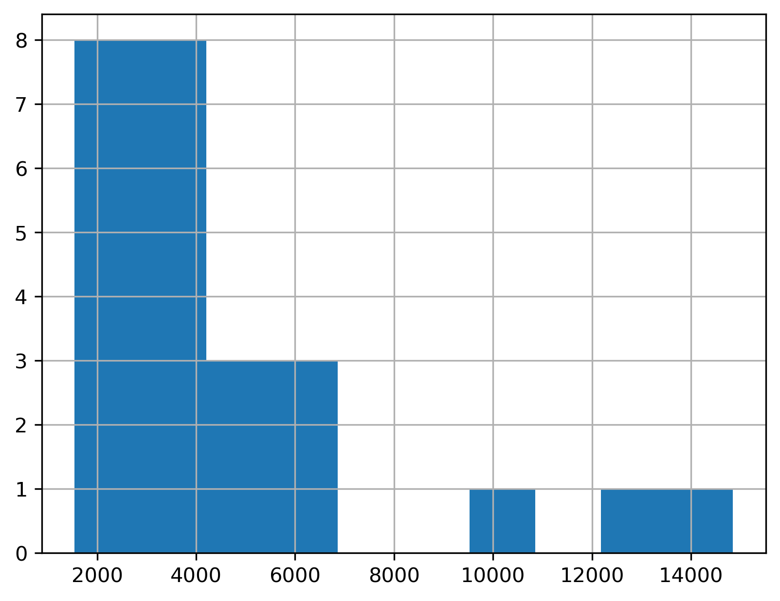
To plot two or more variables, you can use the built-in Pandas bar chart feature.
For example, to plot the GDP of each country in
gdp_americasin 1952 as a bar chart, assign “country” to the x-axis andgdpPerCap_195to the y-axis.
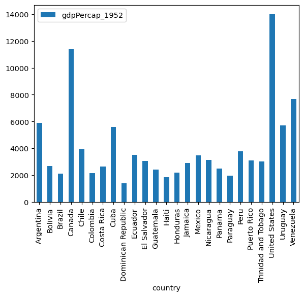
Plotting example: Tracing economic growth
Let’s say you’re only interested in studying the Four Asian Tigers: Hong Kong, Singapore, South Korea, and Taiwan. You want only those rows, and in that order.
To start, let’s read in a version of the gdp_asia data
indexed by country. Then, we can use .loc[] with a list of
rows:
["Singapore", "Taiwan", "Hong Kong China", "Korea Rep."].
Because these are post-war phenomena, you are only interested in
these economies as they have evolved since 1962, so pass in the range
"gdpPercap_1962":"gdpPercap_1997" to
.loc[].
PYTHON
import pandas as pd
gdp_asia_country = pd.read_csv("../data/gapminder_gdp_asia.csv", index_col="country")
tigers = gdp_asia_country.loc[["Singapore", "Taiwan", "Hong Kong China",
"Korea Rep."], "gdpPercap_1962":"gdpPercap_1997"]
tigersOUTPUT
gdpPercap_1962 gdpPercap_1967 gdpPercap_1972 gdpPercap_1977 gdpPercap_1982 gdpPercap_1987 gdpPercap_1992 gdpPercap_1997
country
Singapore 3674.735572 4977.418540 8597.756202 11210.089480 15169.161120 18861.530810 24769.89120 33519.47660
Taiwan 1822.879028 2643.858681 4062.523897 5596.519826 7426.354774 11054.561750 15215.65790 20206.82098
Hong Kong China 4692.648272 6197.962814 8315.928145 11186.141250 14560.530510 20038.472690 24757.60301 28377.63219
Korea Rep. 1536.344387 2029.228142 3030.876650 4657.221020 5622.942464 8533.088805 12104.27872 15993.52796If we try the default parameters (no arguments passed) with
.plot(), we get a graph that’s not quite what we want. The
x and y axes are reversed.
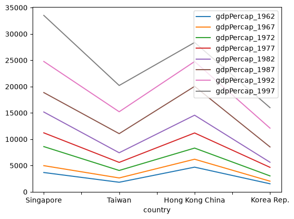
We can address this by plotting the DataFrame using the
.T attribute to flip the x and y axes of the
tigers DataFrame.
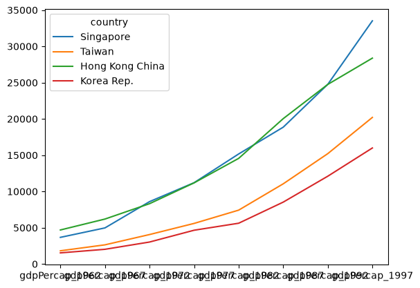
Now, we’ll fix the axes. To adjust the column names, we’ll apply a
special removeprefix
method to remove the gdpPercap_ prefix.
OUTPUT
1962 1967 1972 1977 1982 1987 1992 1997
country
Singapore 3674.735572 4977.418540 8597.756202 11210.089480 15169.161120 18861.530810 24769.89120 33519.47660
Taiwan 1822.879028 2643.858681 4062.523897 5596.519826 7426.354774 11054.561750 15215.65790 20206.82098
Hong Kong China 4692.648272 6197.962814 8315.928145 11186.141250 14560.530510 20038.472690 24757.60301 28377.63219
Korea Rep. 1536.344387 2029.228142 3030.876650 4657.221020 5622.942464 8533.088805 12104.27872 15993.52796Let’s try plotting the transposed version of our modified DataFrame again.
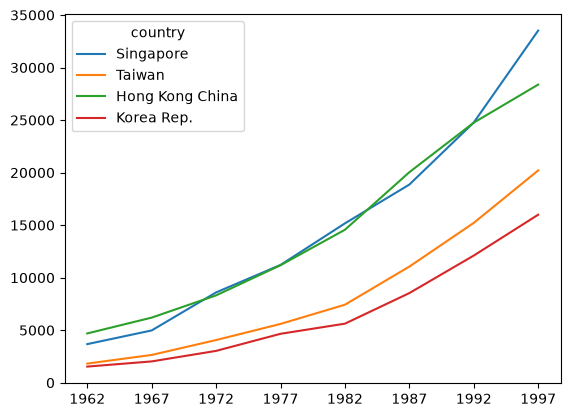
We can combine plotting with other statistic methods by chaining them together. For example, let’s plot the median GDP per capita of the Four Tigers between 1952 and 1997.
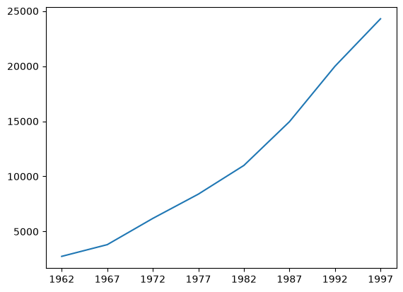
Customizing plots
We can use the plt module from matplotlib
to customize the appearance of our plots.
We can use the plt.xlabel() and
plt.ylabel() functions to label the x and y axes of our
plots.
PYTHON
import matplotlib.pyplot as plt
tigers.T.plot() # Example of "chaining"
plt.ylabel('GDP per capita')
plt.xlabel('Year')
plt.show()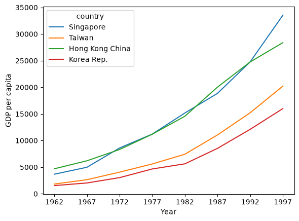
We can also customize the color of our plot. Let’s try a grouped bar chart comparing the GDP per-capita of New Zealand and Australia.
This will require us to read in the
gapminder_gdp_oceania.csv file and apply the same
.removeprefix() we used before.
PYTHON
gdp_oceania = pd.read_csv("data/gapminder_gdp_oceania.csv",
index_col="country")
gdp_oceania.columns = gdp_oceania.columns.str.removeprefix("gdpPercap_")Let’s try plotting the gdp_oceania DataFrame with the
default settings.
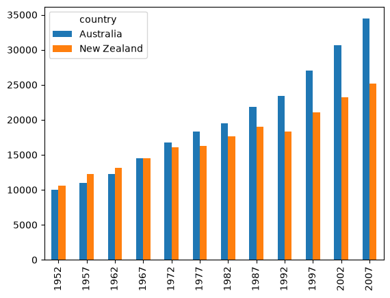
Let’s add a title, axes, and color configuration options. Try turning
the stacked= argument on and off to see what it does!
PYTHON
gdp_oceania.T.plot.bar(color=["orange", "navy"], stacked=True)
plt.title("Oceania Economic Growth")
plt.ylabel('GDP per capita')
plt.xlabel('Year')
plt.show()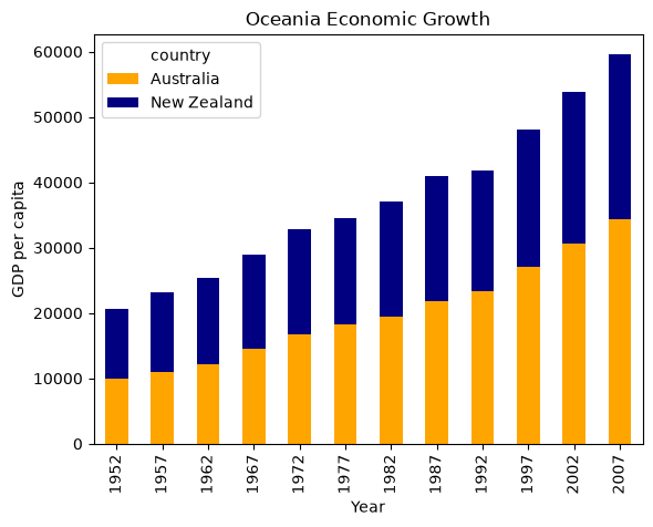
You can learn more about plotting configuration options in the Pandas documentation and the Matplotlib documentation.
Minima and Maxima
Fill in the blanks below to plot the minimum GDP per capita over time for all the countries in Europe. Modify it again to plot the maximum GDP per capita over time for Europe.
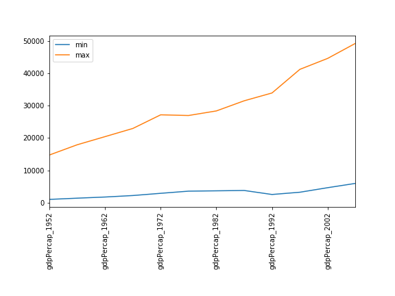

Correlations
Modify the example in the notes to create a scatter plot showing the relationship between the minimum and maximum GDP per capita among the countries in Asia for each year in the data set. What relationship do you see (if any)?
PYTHON
data_asia = pd.read_csv('data/gapminder_gdp_asia.csv', index_col='country')
data_asia.describe().T.plot(kind='scatter', x='min', y='max')
No particular correlations can be seen between the minimum and maximum GDP values year on year. It seems the fortunes of asian countries do not rise and fall together.
Correlations (continued)
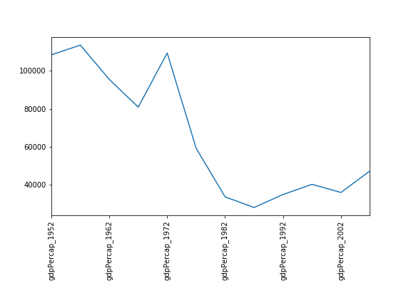
Seems the variability in this value is due to a sharp drop after 1972. Some geopolitics at play perhaps? Given the dominance of oil producing countries, maybe the Brent crude index would make an interesting comparison? Whilst Myanmar consistently has the lowest GDP, the highest GDP nation has varied more notably.
More Correlations
This short program creates a plot showing the correlation between GDP and life expectancy for 2007, normalizing marker size by population:
PYTHON
data_all = pd.read_csv('data/gapminder_all.csv', index_col='country')
data_all.plot(kind='scatter', x='gdpPercap_2007', y='lifeExp_2007',
s=data_all['pop_2007']/1e6)Using online help and other resources, explain what each argument to
plot does.

A good place to look is the documentation for the plot function - help(data_all.plot).
kind - As seen already this determines the kind of plot to be drawn.
x and y - A column name or index that determines what data will be placed on the x and y axes of the plot
s - Details for this can be found in the documentation of plt.scatter. A single number or one value for each data point. Determines the size of the plotted points.
Saving your plot to a file
If you are satisfied with the plot you see you may want to save it to a file, perhaps to include it in a publication. There is a function in the matplotlib.pyplot module that accomplishes this: savefig. Calling this function, e.g. with
will save the current figure to the file my_figure.png.
The file format will automatically be deduced from the file name
extension (other formats are pdf, ps, eps and svg).
Note that functions in plt refer to a global figure
variable and after a figure has been displayed to the screen (e.g. with
plt.show) matplotlib will make this variable refer to a new
empty figure. Therefore, make sure you call plt.savefig
before the plot is displayed to the screen, otherwise you may find a
file with an empty plot.
When using dataframes, data is often generated and plotted to screen
in one line. In addition to using plt.savefig, we can save
a reference to the current figure in a local variable (with
plt.gcf) and call the savefig class method
from that variable to save the figure to file.
Making your plots accessible
Whenever you are generating plots to go into a paper or a presentation, there are a few things you can do to make sure that everyone can understand your plots.
- Always make sure your text is large enough to read. Use the
fontsizeparameter inxlabel,ylabel,title, andlegend, andtick_paramswithlabelsizeto increase the text size of the numbers on your axes. - Similarly, you should make your graph elements easy to see. Use
sto increase the size of your scatterplot markers andlinewidthto increase the sizes of your plot lines. - Using color (and nothing else) to distinguish between different plot
elements will make your plots unreadable to anyone who is colorblind, or
who happens to have a black-and-white office printer. For lines, the
linestyleparameter lets you use different types of lines. For scatterplots,markerlets you change the shape of your points. If you’re unsure about your colors, you can use Coblis or Color Oracle to simulate what your plots would look like to those with colorblindness.
Key Points
-
matplotlibis the most widely used scientific plotting library in Python. - You can plot data directly from a Pandas dataframe using
.plot(). - Many styles of plot are available: see the Python Graph Gallery for more options.
Content from Writing Functions
Last updated on 2024-06-13 | Edit this page
Overview
Questions
- How can I create my own functions?
Objectives
- Explain and identify the difference between function definition and function call.
- Write a function that takes a small, fixed number of arguments and produces a single result.
Break programs down into functions to make them easier to understand.
- Human beings can only keep a few items in working memory at a time.
- Understand larger/more complicated ideas by understanding and
combining pieces.
- Components in a machine.
- Lemmas when proving theorems.
- Functions serve the same purpose in programs.
- Encapsulate complexity so that we can treat it as a single “thing”.
- Also enables re-use.
- Write one time, use many times.
Define a function using def with a name, parameters,
and a block of code.
- Begin the definition of a new function with
def. - Followed by the name of the function.
- Must obey the same rules as variable names.
- Then parameters in parentheses.
- Empty parentheses if the function doesn’t take any inputs.
- We will discuss this in detail in a moment.
- Then a colon.
- Then an indented block of code.
Defining a function does not run it.
- Defining a function does not run it.
- Like assigning a value to a variable.
- Must call the function to execute the code it contains.
OUTPUT
Hello!Arguments in a function call are matched to its defined parameters.
- Functions are most useful when they can operate on different data.
- Specify parameters when defining a function.
- These become variables when the function is executed.
- Are assigned the arguments in the call (i.e., the values passed to the function).
- If you don’t name the arguments when using them in the call, the arguments will be matched to parameters in the order the parameters are defined in the function.
PYTHON
def print_date(year, month, day):
joined = str(year) + '/' + str(month) + '/' + str(day)
print(joined)
print_date(1871, 3, 19)OUTPUT
1871/3/19Or, we can name the arguments when we call the function, which allows us to specify them in any order and adds clarity to the call site; otherwise as one is reading the code they might forget if the second argument is the month or the day for example.
OUTPUT
1871/3/19- Via Twitter:
()contains the ingredients for the function while the body contains the recipe.
Functions may return a result to their caller using
return.
- Use
return ...to give a value back to the caller. - May occur anywhere in the function.
- But functions are easier to understand if
returnoccurs:- At the start to handle special cases.
- At the very end, with a final result.
OUTPUT
average of actual values: 2.6666666666666665OUTPUT
average of empty list: None- Remember: every function returns something.
- A function that doesn’t explicitly
returna value automatically returnsNone.
OUTPUT
1871/3/19
result of call is: NoneIdentifying Syntax Errors
- Read the code below and try to identify what the errors are without running it.
- Run the code and read the error message. Is it a
SyntaxErroror anIndentationError? - Fix the error.
- Repeat steps 2 and 3 until you have fixed all the errors.
OUTPUT
calling <function report at 0x7fd128ff1bf8> 22.5A function call always needs parenthesis, otherwise you get memory address of the function object. So, if we wanted to call the function named report, and give it the value 22.5 to report on, we could have our function call as follows
OUTPUT
calling
pressure is 22.5Order of Operations
- What’s wrong in this example?
PYTHON
result = print_time(11, 37, 59)
def print_time(hour, minute, second):
time_string = str(hour) + ':' + str(minute) + ':' + str(second)
print(time_string)- After fixing the problem above, explain why running this example code:
gives this output:
OUTPUT
11:37:59
result of call is: None- Why is the result of the call
None?
The problem with the example is that the function
print_time()is defined after the call to the function is made. Python doesn’t know how to resolve the nameprint_timesince it hasn’t been defined yet and will raise aNameErrore.g.,NameError: name 'print_time' is not definedThe first line of output
11:37:59is printed by the first line of code,result = print_time(11, 37, 59)that binds the value returned by invokingprint_timeto the variableresult. The second line is from the second print call to print the contents of theresultvariable.print_time()does not explicitlyreturna value, so it automatically returnsNone.
Find the First
Calling by Name
Earlier we saw this function:
PYTHON
def print_date(year, month, day):
joined = str(year) + '/' + str(month) + '/' + str(day)
print(joined)We saw that we can call the function using named arguments, like this:
- What does
print_date(day=1, month=2, year=2003)print? - When have you seen a function call like this before?
- When and why is it useful to call functions this way?
2003/2/1- We saw examples of using named arguments when working with
the pandas library. For example, when reading in a dataset using
data = pd.read_csv('data/gapminder_gdp_europe.csv', index_col='country'), the last argumentindex_colis a named argument. - Using named arguments can make code more readable since one can see from the function call what name the different arguments have inside the function. It can also reduce the chances of passing arguments in the wrong order, since by using named arguments the order doesn’t matter.
Encapsulation of an If/Print Block
The code below will run on a label-printer for chicken eggs. A digital scale will report a chicken egg mass (in grams) to the computer and then the computer will print a label.
PYTHON
import random
for i in range(10):
# simulating the mass of a chicken egg
# the (random) mass will be 70 +/- 20 grams
mass = 70 + 20.0 * (2.0 * random.random() - 1.0)
print(mass)
# egg sizing machinery prints a label
if mass >= 85:
print("jumbo")
elif mass >= 70:
print("large")
elif mass < 70 and mass >= 55:
print("medium")
else:
print("small")The if-block that classifies the eggs might be useful in other
situations, so to avoid repeating it, we could fold it into a function,
get_egg_label(). Revising the program to use the function
would give us this:
PYTHON
# revised version
import random
for i in range(10):
# simulating the mass of a chicken egg
# the (random) mass will be 70 +/- 20 grams
mass = 70 + 20.0 * (2.0 * random.random() - 1.0)
print(mass, get_egg_label(mass))- Create a function definition for
get_egg_label()that will work with the revised program above. Note that theget_egg_label()function’s return value will be important. Sample output from the above program would be71.23 large. - A dirty egg might have a mass of more than 90 grams, and a spoiled
or broken egg will probably have a mass that’s less than 50 grams.
Modify your
get_egg_label()function to account for these error conditions. Sample output could be25 too light, probably spoiled.
PYTHON
def get_egg_label(mass):
# egg sizing machinery prints a label
egg_label = "Unlabelled"
if mass >= 90:
egg_label = "warning: egg might be dirty"
elif mass >= 85:
egg_label = "jumbo"
elif mass >= 70:
egg_label = "large"
elif mass < 70 and mass >= 55:
egg_label = "medium"
elif mass < 50:
egg_label = "too light, probably spoiled"
else:
egg_label = "small"
return egg_labelEncapsulating Data Analysis
Assume that the following code has been executed:
PYTHON
import pandas as pd
data_asia = pd.read_csv('data/gapminder_gdp_asia.csv', index_col=0)
japan = data_asia.loc['Japan']- Complete the statements below to obtain the average GDP for Japan across the years reported for the 1980s.
PYTHON
year = 1983
gdp_decade = 'gdpPercap_' + str(year // ____)
avg = (japan.loc[gdp_decade + ___] + japan.loc[gdp_decade + ___]) / 2- Abstract the code above into a single function.
PYTHON
def avg_gdp_in_decade(country, continent, year):
data_countries = pd.read_csv('data/gapminder_gdp_'+___+'.csv',delimiter=',',index_col=0)
____
____
____
return avg- How would you generalize this function if you did not know beforehand which specific years occurred as columns in the data? For instance, what if we also had data from years ending in 1 and 9 for each decade? (Hint: use the columns to filter out the ones that correspond to the decade, instead of enumerating them in the code.)
- The average GDP for Japan across the years reported for the 1980s is computed with:
PYTHON
year = 1983
gdp_decade = 'gdpPercap_' + str(year // 10)
avg = (japan.loc[gdp_decade + '2'] + japan.loc[gdp_decade + '7']) / 2- That code as a function is:
PYTHON
def avg_gdp_in_decade(country, continent, year):
data_countries = pd.read_csv('data/gapminder_gdp_' + continent + '.csv', index_col=0)
c = data_countries.loc[country]
gdp_decade = 'gdpPercap_' + str(year // 10)
avg = (c.loc[gdp_decade + '2'] + c.loc[gdp_decade + '7'])/2
return avg- To obtain the average for the relevant years, we need to loop over them:
PYTHON
def avg_gdp_in_decade(country, continent, year):
data_countries = pd.read_csv('data/gapminder_gdp_' + continent + '.csv', index_col=0)
c = data_countries.loc[country]
gdp_decade = 'gdpPercap_' + str(year // 10)
total = 0.0
num_years = 0
for yr_header in c.index: # c's index contains reported years
if yr_header.startswith(gdp_decade):
total = total + c.loc[yr_header]
num_years = num_years + 1
return total/num_yearsThe function can now be called by:
OUTPUT
20880.023800000003Simulating a dynamical system
In mathematics, a dynamical system is a system in which a function describes the time dependence of a point in a geometrical space. A canonical example of a dynamical system is the logistic map, a growth model that computes a new population density (between 0 and 1) based on the current density. In the model, time takes discrete values 0, 1, 2, …
- Define a function called
logistic_mapthat takes two inputs:x, representing the current population (at timet), and a parameterr = 1. This function should return a value representing the state of the system (population) at timet + 1, using the mapping function:
f(t+1) = r * f(t) * [1 - f(t)]
Using a
fororwhileloop, iterate thelogistic_mapfunction defined in part 1, starting from an initial population of 0.5, for a period of timet_final = 10. Store the intermediate results in a list so that after the loop terminates you have accumulated a sequence of values representing the state of the logistic map at timest = [0,1,...,t_final](11 values in total). Print this list to see the evolution of the population.Encapsulate the logic of your loop into a function called
iteratethat takes the initial population as its first input, the parametert_finalas its second input and the parameterras its third input. The function should return the list of values representing the state of the logistic map at timest = [0,1,...,t_final]. Run this function for periodst_final = 100and1000and print some of the values. Is the population trending toward a steady state?
-
PYTHON
def iterate(initial_population, t_final, r): population = [initial_population] for t in range(t_final): population.append( logistic_map(population[t], r) ) return population for period in (10, 100, 1000): population = iterate(0.5, period, 1) print(population[-1])The population seems to be approaching zero.OUTPUT
0.06945089389714401 0.009395779870614648 0.0009913908614406382
Using Functions With Conditionals in Pandas
Functions will often contain conditionals. Here is a short example that will indicate which quartile the argument is in based on hand-coded values for the quartile cut points.
PYTHON
def calculate_life_quartile(exp):
if exp < 58.41:
# This observation is in the first quartile
return 1
elif exp >= 58.41 and exp < 67.05:
# This observation is in the second quartile
return 2
elif exp >= 67.05 and exp < 71.70:
# This observation is in the third quartile
return 3
elif exp >= 71.70:
# This observation is in the fourth quartile
return 4
else:
# This observation has bad data
return None
calculate_life_quartile(62.5)OUTPUT
2That function would typically be used within a for loop,
but Pandas has a different, more efficient way of doing the same thing,
and that is by applying a function to a dataframe or a portion
of a dataframe. Here is an example, using the definition above.
PYTHON
data = pd.read_csv('data/gapminder_all.csv')
data['life_qrtl'] = data['lifeExp_1952'].apply(calculate_life_quartile)There is a lot in that second line, so let’s take it piece by piece.
On the right side of the = we start with
data['lifeExp'], which is the column in the dataframe
called data labeled lifExp. We use the
apply() to do what it says, apply the
calculate_life_quartile to the value of this column for
every row in the dataframe.
Key Points
- Break programs down into functions to make them easier to understand.
- Define a function using
defwith a name, parameters, and a block of code. - Defining a function does not run it.
- Arguments in a function call are matched to its defined parameters.
- Functions may return a result to their caller using
return.
Content from Variable Scope
Last updated on 2023-05-02 | Edit this page
Overview
Questions
- How do function calls actually work?
- How can I determine where errors occurred?
Objectives
- Identify local and global variables.
- Identify parameters as local variables.
- Read a traceback and determine the file, function, and line number on which the error occurred, the type of error, and the error message.
The scope of a variable is the part of a program that can ‘see’ that variable.
- There are only so many sensible names for variables.
- People using functions shouldn’t have to worry about what variable names the author of the function used.
- People writing functions shouldn’t have to worry about what variable names the function’s caller uses.
- The part of a program in which a variable is visible is called its scope.
-
pressureis a global variable.- Defined outside any particular function.
- Visible everywhere.
-
tandtemperatureare local variables inadjust.- Defined in the function.
- Not visible in the main program.
- Remember: a function parameter is a variable that is automatically assigned a value when the function is called.
OUTPUT
adjusted: 0.01238691049085659ERROR
Traceback (most recent call last):
File "/Users/swcarpentry/foo.py", line 8, in <module>
print('temperature after call:', temperature)
NameError: name 'temperature' is not definedReading Error Messages
Read the traceback below, and identify the following:
- How many levels does the traceback have?
- What is the file name where the error occurred?
- What is the function name where the error occurred?
- On which line number in this function did the error occur?
- What is the type of error?
- What is the error message?
ERROR
---------------------------------------------------------------------------
KeyError Traceback (most recent call last)
<ipython-input-2-e4c4cbafeeb5> in <module>()
1 import errors_02
----> 2 errors_02.print_friday_message()
/Users/ghopper/thesis/code/errors_02.py in print_friday_message()
13
14 def print_friday_message():
---> 15 print_message("Friday")
/Users/ghopper/thesis/code/errors_02.py in print_message(day)
9 "sunday": "Aw, the weekend is almost over."
10 }
---> 11 print(messages[day])
12
13
KeyError: 'Friday'- Three levels.
errors_02.pyprint_message- Line 11
-
KeyError. These errors occur when we are trying to look up a key that does not exist (usually in a data structure such as a dictionary). We can find more information about theKeyErrorand other built-in exceptions in the Python docs. KeyError: 'Friday'
Key Points
- The scope of a variable is the part of a program that can ‘see’ that variable.
Content from Programming Style
Last updated on 2023-07-29 | Edit this page
Overview
Questions
- How can I make my programs more readable?
- How do most programmers format their code?
- How can programs check their own operation?
Objectives
- Provide sound justifications for basic rules of coding style.
- Refactor one-page programs to make them more readable and justify the changes.
- Use Python community coding standards (PEP-8).
Coding style
A consistent coding style helps others (including our future selves) read and understand code more easily. Code is read much more often than it is written, and as the Zen of Python states, “Readability counts”. Python proposed a standard style through one of its first Python Enhancement Proposals (PEP), PEP8.
Some points worth highlighting:
- document your code and ensure that assumptions, internal algorithms, expected inputs, expected outputs, etc., are clear
- use clear, semantically meaningful variable names
- use white-space, not tabs, to indent lines (tabs can cause problems across different text editors, operating systems, and version control systems)
Follow standard Python style in your code.
-
PEP8: a style
guide for Python that discusses topics such as how to name variables,
how to indent your code, how to structure your
importstatements, etc. Adhering to PEP8 makes it easier for other Python developers to read and understand your code, and to understand what their contributions should look like. - To check your code for compliance with PEP8, you can use the pycodestyle application and tools like the black code formatter can automatically format your code to conform to PEP8 and pycodestyle (a Jupyter notebook formatter also exists nb_black).
- Some groups and organizations follow different style guidelines besides PEP8. For example, the Google style guide on Python makes slightly different recommendations. Google wrote an application that can help you format your code in either their style or PEP8 called yapf.
- With respect to coding style, the key is consistency. Choose a style for your project be it PEP8, the Google style, or something else and do your best to ensure that you and anyone else you are collaborating with sticks to it. Consistency within a project is often more impactful than the particular style used. A consistent style will make your software easier to read and understand for others and for your future self.
Use assertions to check for internal errors.
Assertions are a simple but powerful method for making sure that the context in which your code is executing is as you expect.
PYTHON
def calc_bulk_density(mass, volume):
'''Return dry bulk density = powder mass / powder volume.'''
assert volume > 0
return mass / volumeIf the assertion is False, the Python interpreter raises
an AssertionError runtime exception. The source code for
the expression that failed will be displayed as part of the error
message. To ignore assertions in your code run the interpreter with the
‘-O’ (optimize) switch. Assertions should contain only simple checks and
never change the state of the program. For example, an assertion should
never contain an assignment.
Use docstrings to provide builtin help.
If the first thing in a function is a character string that is not assigned directly to a variable, Python attaches it to the function, accessible via the builtin help function. This string that provides documentation is also known as a docstring.
PYTHON
def average(values):
"Return average of values, or None if no values are supplied."
if len(values) == 0:
return None
return sum(values) / len(values)
help(average)OUTPUT
Help on function average in module __main__:
average(values)
Return average of values, or None if no values are supplied.What Will Be Shown?
Highlight the lines in the code below that will be available as online help. Are there lines that should be made available, but won’t be? Will any lines produce a syntax error or a runtime error?
PYTHON
"Find maximum edit distance between multiple sequences."
# This finds the maximum distance between all sequences.
def overall_max(sequences):
'''Determine overall maximum edit distance.'''
highest = 0
for left in sequences:
for right in sequences:
'''Avoid checking sequence against itself.'''
if left != right:
this = edit_distance(left, right)
highest = max(highest, this)
# Report.
return highestDocument This
Use comments to describe and help others understand potentially unintuitive sections or individual lines of code. They are especially useful to whoever may need to understand and edit your code in the future, including yourself.
Use docstrings to document the acceptable inputs and expected outputs
of a method or class, its purpose, assumptions and intended behavior.
Docstrings are displayed when a user invokes the builtin
help method on your method or class.
Turn the comment in the following function into a docstring and check
that help displays it properly.
Clean Up This Code
- Read this short program and try to predict what it does.
- Run it: how accurate was your prediction?
- Refactor the program to make it more readable. Remember to run it after each change to ensure its behavior hasn’t changed.
- Compare your rewrite with your neighbor’s. What did you do the same? What did you do differently, and why?
Here’s one solution.
PYTHON
def string_machine(input_string, iterations):
"""
Takes input_string and generates a new string with -'s and *'s
corresponding to characters that have identical adjacent characters
or not, respectively. Iterates through this procedure with the resultant
strings for the supplied number of iterations.
"""
print(input_string)
input_string_length = len(input_string)
old = input_string
for i in range(iterations):
new = ''
# iterate through characters in previous string
for j in range(input_string_length):
left = j-1
right = (j+1) % input_string_length # ensure right index wraps around
if old[left] == old[right]:
new = new + '-'
else:
new = new + '*'
print(new)
# store new string as old
old = new
string_machine('et cetera', 10)OUTPUT
et cetera
*****-***
----*-*--
---*---*-
--*-*-*-*
**-------
***-----*
--**---**
*****-***
----*-*--
---*---*-Key Points
- Follow standard Python style in your code.
- Use docstrings to provide builtin help.
Content from Wrap-Up
Last updated on 2023-05-02 | Edit this page
Overview
Questions
- What have we learned?
- What else is out there and where do I find it?
Objectives
- Name and locate scientific Python community sites for software, workshops, and help.
Leslie Lamport once said, “Writing is nature’s way of showing you how sloppy your thinking is.” The same is true of programming: many things that seem obvious when we’re thinking about them turn out to be anything but when we have to explain them precisely.
Python supports a large and diverse community across academia and industry.
The Python 3 documentation covers the core language and the standard library.
PyCon is the largest annual conference for the Python community.
SciPy is a rich collection of scientific utilities. It is also the name of a series of annual conferences.
Jupyter is the home of Project Jupyter.
Pandas is the home of the Pandas data library.
Stack Overflow’s general Python section can be helpful, as well as the sections on NumPy, SciPy, and Pandas.
Key Points
- Python supports a large and diverse community across academia and industry.